An Introduction to Nonparametric Regression
320 likes | 953 Vues
An Introduction to Nonparametric Regression. Ning Li March 15 th , 2004 Biostatistics 277. Reference. Applied Nonparametric Regression, Wolfgang Hardle, Cambridge 1994. Chapter 1 – 3. . Outline. Introduction Motivation Basic Idea of Smoothing Smoothing techniques Kernel smoothing

An Introduction to Nonparametric Regression
E N D
Presentation Transcript
An Introduction to Nonparametric Regression Ning Li March 15th, 2004 Biostatistics 277
Reference • Applied Nonparametric Regression, Wolfgang Hardle, Cambridge 1994. Chapter 1 – 3.
Outline • Introduction • Motivation • Basic Idea of Smoothing • Smoothing techniques Kernel smoothing k-nearest neighbor estimates spline smoothing • A comparison of kernel, k-NN and spline smoothers
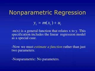
Introduction • The aim of a regression analysis is to produce a reasonable analysis to the unknown response function m, where for n data points ( ), the relationship can be modeled as • Unlike parametric approach where the function m is fully described by a finite set of parameters, nonparametric modeling accommodate a very flexible form of the regression curve.
Motivation • It provides a versatile method of exploring a general relationship between variables • It gives predictions of observations yet to be made without reference to a fixed parametric model • It provides a tool for finding spurious observations by studying the influence of isolated points • It constitutes a flexible method of substituting for missing values or interpolating between adjacent X-values
Basic Idea of Smoothing • A reasonable approximation to the regression curve m(x) will be the mean of response variables near a point x. This local averaging procedure can be defined as Every smoothing method to be described is of the form (2). • The amount of averaging is controlled by a smoothing parameter. The choice of smoothing parameter is related to the balances between bias and variance.
Figure 1. Expenditure of potatoes as a function of net income. h = 0.1, 1.0, n = 7125, year = 1973.
Smoothing TechniquesKernel Smoothing • Kernel smoothing describes the shape of the weight function by a density function K with a scale parameter that adjusts the size and the form of the weights near x. The kernelK is a continuous, bounded and symmetric real function which integrates to 1. The weight is defined by where , and .
Kernel Smoothing • The Nadaraya-Watson estimator is defined by The mean squared error is . As we have, under certain conditions, Where The bias is increasing whereas the variance is decreasing in h.
Figure 2. The Epanechnikov kernel K (u) = 0.75(1-u2) I (|u| <= 1 ).
Figure 3. The effective kernel weights for the food versus net income data set. at x = 1 and x = 2.5 for h = 0.1 ( label 1 ), h = 0.2 ( label 2 ), h = 0.3 ( label 3 ) with Epanechnikov kernel.
K-Nearest Neighbor Estimates • In k-NN, the neighborhood is defined through those X – variables which are among the k-nearest neighbors of x in Euclidean distance. The k-NN smoother is defined as where { } i=1, …, n is defined through the set of Indexes , and
K-nearest Neighbor Estimates • The smoothing parameter k regulates the degree of smoothness of the estimated curve. It plays a role similar to the bandwidth for kernel smoothers. • The influence of varying k on qualitative features of the estimated curve is similar to that observed for kernel estimation with a uniform kernel. • When k > n, the k - NN smoother then is equal to the average of the response variables. When k = 1, the observations are reproduced at Xi, and for an x between two adjacent predictor variables a step function is obtained with a jump in the middle between the two observations.
K-nearest Neighbor Estimates • Let . Bias and variance of the k-NN estimate with weights as in (7) are given by Note: The trade-off between bias2 and variance is thus achieved in an asymptotic sense by settingk ~ n4/5
K-nearest Neighbor Estimates • In addition to the “uniform” weights, the k-NN weights can be generally thought of as being generated by a kernel function K, where and R is the distance between x and its k-th nearest neighbor.
Figure 4. The effective k-NN weights for the food versus net income data set. at x = 1 and x = 2.5 for k = 100 ( label 1 ), k = 200 ( label 2 ), k = 300 ( label 3 ) with Epanechnikov kernel.
K-nearest Neighbor Estimates • Let , and cK, dK be defined as previously, then Note: The trade-off between bias2 and variance is thus achieved in an asymptotic sense by settingk ~ n4/5, like the uniform k-NN weights.
Spline Smoothing • Spline smoothing quantifies the competition between •the aim to produce a good fit to the data • the aim to produce a curve without too much rapid local variation. • The regression curve is obtained by minimizing the penalized sum of squares where m is twice-differentiable function on [a,b], and λ represents the rate of exchange between residual error and roughness of the curve m.
Spline Smoothing • The spline is linear in the Y observations, and there exists weights that • Silverman in 1984 showed for large n, small λ, and Xinot too close to the boundary, where the local bandwith h(Xi) satisfies
Spline Smoothing • A variation to (11) is to solve the equivalent problem under the constraint . • The parameters λ and Δ have similar meanings, and are connected by the relationship where and solves (12).
A comparison of kernel, k-NN and spline smoothers Table 1. Bias and variance of kernel and k-NN smoother
Figure 7. A simulated data set. The raw data n=100 were constructed from and
Figure 8. A kernel smooth of the simulated data set. The black line (label 1) denotes the underlying regression curve The green line (label 2) is the Gaussian kernel smooth .
Figure 9. A k-NN kernel smooth of the simulated data set. The black line (label 1) denotes the underlying regression curve. The green line (label 2) is the k-NN smoother
Figure 10. A spline smooth of the simulated data set. The black line (label 1) denotes the underlying regression curve. The green line (label 2) is the spline smoother
Figure 11. Residual plot of k-NN, kernel and spline smoother for the simulated data set.