6. Introduction to nonparametric clustering

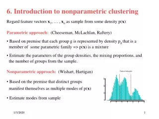
1. 6. Introduction to nonparametric clustering • Regard feature vectors x1, … , xn as sample from some density p(x) • Parametric approach: (Cheeseman, McLachlan, Raftery) • Based on premise that each group g is represented by density pg that is a member of some parametric family => p(x) is a mixture • Estimate the parameters of the group densities, the mixing proportions, and the number of groups from the sample. • Nonparametric approach: (Wishart, Hartigan) • Based on the premise that distinct groups manifest themselves as multiple modes of p(x) • Estimate modes from sample

2. 6.1 Describing the modal structure of a density Consider feature vectors x1 , …. , xn as a sample from some density p(x) . Define level set L(c ; p) as the subset of feature space for which the density p(x) is greater than c. Note: Level sets with multiple connected components indicate multi-modality There might not be a single level set that reveals all the modes

3. The cluster tree of a density • Modal structure of density is described by cluster tree. • Each node N of cluster tree • represents a subset D(N) of feature space • is associated with a density level c(N) • Root node • represents the entire feature space • is associated with density level c(N) = 0 • Tree defined recursively: to determine descendents of node N • Find lowest level c for which intersection of D(N) with L(c ; p) has two connected components • If there is no such c then N is leaf of tree; leaves of tree <==> modes • Otherwise, create daughter nodes representing the connected components, with associated level c

4. Goal: Estimate the cluster tree of the underlying density p(x) from the sample feature vectors x1 , …. , xn First step:Estimate p(x) by density estimate p*(x) (see below) Second step:Compute cluster tree of p* (maybe approximately)

5. 6.2 Density estimation Consider feature vectors x1 , …. , xn as a sample from some density p(x). Goal: Estimate p(x) Simplest idea: Let S(x, r) denote a sphere in feature space with radius r, centered at x. Assuming density is roughly constant over S(x, r), the expected number of sample points inS(x, r) is k ~ n * Volume ( S(x, r) ) * p(x), giving p(x) ~ k / (n * Volume ( S(x, r) ) Kernel estimate: Fix radius r ; k = # of sample feature vectors in S(x, r) K-near-neighbor estimate: Fix count k; r = smallest radius for which S(x, r) contains k sample feature vectors Many refinements have been suggested

6. Example - kernel density estimate in 2-d • Swept under the rug: • Choice of sphere radius r (for kernel estimate) or count k (for near-neighbor estimate) --- critical !! There are automatic methods. • Down-weight observations depending on distance from query point • Adaptive estimation --- vary radius r depending on density • Other types of estimates, etc, etc, etc (extensive literature)

7. Computational complexity • Computing kernel or near-neighbor estimate at query point x requires finding nearest neighbors of x in sample x1 , …. , xn. • Can find k nearest neighbors of x in time ~ log n using spatial partitioning schemes such as k-d trees, after n log n pre-processing • However • Spatial partitioning most effective if n large relative to d. • Theoretical analysis shows that number of nearest neighbors should increase with n and decrease with dimensionality d: k ~ n ^ (4 / (d + 4)). Relevance ? • In low dimensions (d <= 4) can use histogram or average shifted histogram density estimates based on regular binning. • Evaluation for query point in constant time, after pre-processing ~ n • High dimensionality may present problem

8. 6.3 Recursive algorithms for constructing a cluster tree • For most density estimates p*(x), computing level sets and finding their connected components is a daunting problem --- especially in high dimensions. • Idea: Computesample cluster tree instead • Each node N of sample cluster tree • represents a subset X(N) of the sample • is associated with a density level c(N) • Root node • represents the entire sample • is associated with density level c(N) = 0

9. To determine descendents of node N • Find lowest level c for which the intersection of X(N) with L(c ; p*) falls into two connected components Note: Intersection of X(N) with L(c ; p*) consists of those feature vectors in the node N for which estimated density p*(xi) > c. @ • If there is no such c then N is leaf of tree; • Otherwise, create daughter nodes representing the “connected components”, with associated level c. • Note: • @ is the critical step. Will in general have to rely on heuristic. • Daughters of a node N do not define a partition of X(N). Assigning low density observations in X(N) to one of the daughters is supervised learning problem

10. Illustration

11. Critical step • Find lowest level c for which observations in X(N) with estimated density p*(xi) > c fall into two connected components of level set L(c ; p*) • Heuristic 1 :(goes with k-near-neighbor density estimate) • Select feature vectors xiin X(N) withp*(xi) > c • Generate graph connecting each feature vector to its k nearest neighbors • Check whether graph has 1 or 2 connected components • Heuristic 2 :(goes with kernel density estimate) • Select feature vectors xiin X(N) withp*(xi) > c • Generate graph connecting feature vectors with distance < r • Check whether graph has 1 or 2 connected components

12. 6.4 Related work / references • Looking for the connected components of a level set --- One-level Mode Analysis --- was first suggested by David Wishart (1969). • Wishart’s paper appeared in obscure place --- Proceedings of the Colloquium in Numerical Taxonomy, St. Andrews, 1968. Nobody in CS cites Wishart. • Idea has been re-invented multiple times --- “sharpening” (Tukey & Tukey); DBSCAN (Ester et al)… Methods differ in heuristics for finding connected components of level set. • Wishart also realized that looking at single level set might not be enough to detect all the modes ==> Hierarchical Mode Analysis. Did not think of it as estimating cluster tree. Algorithm awkward --- based on iterative merging instead of recursive partitioning.OPTICS method of Ankerst et al also considers level sets for different levels.