Download
1 / 43
430 likes | 516 Vues
Learn the basics of simple linear regression, including finding relationships between variables and using SPSS for analysis. Understand regression models, error terms, residuals, and coefficient interpretation. Explore measures of variation, coefficient of determination, and inference techniques. Enhance your statistical analysis skills with practical examples and insights.

E N D
Introduction to linear regression • Simple linear regression • Multiple regression • Find out relationships between dependent and independent variable • Introduction to SPSS
Simple linear regression y = Dependent variable X = Independent variable = y-intercept of the line (constant), cuts through the y-axis = Unknown parameter – Slope of the line = Random error component
Examples • With a sample from the population • denote a random sample of size n from the population File: dataspss-s4.1
DETERMINING THE EQUATION OF THE REGRESSION LINE • Deterministic Regression Model – mathematical models that produce an ‘exact’ output for a given input • Probabilistic Regression Model- a model that includes an error term that allows for various values of output to occur for a given value of input = predicted value of y = value of independent variable for the ith value = realvalue of dependent variable for the ith value = population slope = population intercept = error of prediction for the ithvalue
Simple Linear Regression Model Y Observed value of Y for Xi εi Slope = β1 Predicted value of Y for Xi Random error for this Xi value Intercept = β0 X Xi
SampleRegression Function (SRF) = estimated value of Y for observation i xi = value of X for observation i b0 = Y- intercept is the value of Y when X is zero b1 = slope of the regression line change in Y for 1 unit X b1 > 0 : Line will go up; positive relationship between X and Y b1 < 0 : Line will go down; negative relationship between X and Y
SIMPLE LINEAR REGRESSION MODEL (sample) Simple Linear Regression: where
Sample Regression Function (SRF) (continued) • b0and b1are obtained by finding the values of b0 and b1 that minimizes the sum of the squared residuals (minimize the error). This process is called Least Squares Analysis • b0 provides an estimate of 0 • b1provides and estimate of 1 Yi = actual value of Y for observation i = predicted value of Y for observation i ei = residual (error)
RESIDUAL ANALYSIS • Residual :Difference between the actual y value and the predicted y values predicted by the regression model • Sum of the residuals is zero
Simple example X = experience years (year) Y = Income (10 million VND)
Fit to the data y . 4 3 . . 2 . . 1 x 4 5 2 3 1
Meaning of b0and b1 • Y-Intercept (b0) • Average value of individual income (Y) is -0.1 (10 million VND) when when the experience year (X) is 0 • Slope (b1) • Income (Y) is expected to increase by 0.7 (*10 million VND) for each unit increased in experience year b1 > 0 : Line will go up; positive relationship between X and Y (increase) b1 < 0 : Line will go down; negative relationship between X and Y (decrease)
Measures of Variation Total variation is made up of two parts. Error Sum of Squares Regression Sum of Squares Total Sum of Squares Variation attributable to factors other than the relationship between X and Y. Measures the variation of the Yi values around their mean Y. Explained variation attributable to the relationship between X and Y. /* Other notation for SSyy is SST. They are the same!
Measure of Variation: The Sum of Squares (continued) Y SSE =(Yi-Yi )2 _ SSyy=(Yi-Y)2 _ SSR = (Yi -Y)2 _ Y X Xi
Coefficient of Determination, r2 The coefficient of determination is the portion of the total variation in the dependent variable that is explained by variation in the independent variable. The coefficient of determination is also called r-squared and is denoted as r2 Note:
The Coefficient of Determinationr2 and the Coefficient of Correlationr r2 = Coefficient of Determination Measures the % of variation in Y that is explained by the independent variable X in the regression model r = Coefficient of Correlation Measures how strong the relationship is between X and Y r > 0 if b1>0 r < 0 if b1 <0 0<r2<1 -1<r<1
Examples of Approximate r2 values Perfect linear relationship between X and Y. 100% of the variation in Y is explained by variation in X. Y Y X X r2 = 1 r2 = 1 Y No linear relationship between X and Y. The value of Y does not depend on X (None of the variation in Y is explained by variation in X). X r2 = 0
Examples of Approximate r2 values 0 < r2 < 1 Y Weaker linear relationships between X and Y. Some but not all of the variation in Y is explained by variation in X. X Y X
Standard Error of the Estimate The standard deviation of the variation of observations around the regression line is estimated by: Where SSE = error sum of squares n = sample size
Inferences About the Slope The standard error of the regression slope coefficient (b1) is estimated by: Where = Estimate of the standard error of the least squares slope. = Standard error of the estimate.
Result of estimation by SPSS Sb1 = 0.1914854
Inference about the Slope: t Test t test for a population slope: • Is there a linear relationship between X and Y? Null hypothesis (H0) and Alternative hypothesis (H1) H0: β1 = 0 (no linear relationship) H1: β1 ≠ 0 (linear relationship does exist) Test statistic with d.f. = n-2 Where b1 = regression slope coefficient β1 = hypothesized slope Sb1 = standard error of the slope
Inferences about the Slope: tTest Example H0: β1 = 0 H1: β1 ≠0 Test Statistic: t = 3.66 T critical = +/- 3.182 (from t tables) Decision: Reject H0 Conclusion: There is sufficient evidence that number of customers affects weekly sales. d.f. = 5-2 = 3 /2=.025 Do not reject H0 /2=.025 Reject H0 Reject H0 -t/2 t/2 0 -3.182 3.182 3.66
F Test for Significance F Test statistic: Where F follows an F distribution with k numerator and (n – k - 1) denominator degrees of freedom. k = the number of independent (explanatory) variables in the regression model.
F Test for Significance Example df1= k =1 df2 = n-k-1=5-1-1 Test Statistic: Conclusion: Reject H0 at = 0.05 There is sufficient evidence that number of customers affects weekly sales. H0: β1 = 0 H1: β1 ≠ 0 = .05 df1= 1 df2 = 3 Critical Value: F = 10.128 = .05 0 F Do not reject H0 Reject H0 F.05 = 10.128
Voice of result • R-squared ranges in value between 0 and 1 • R2 = 0, nothing to help explain the variance in y • R2 = 1, all the same points lie on the estimated regression line • Example: R2 = 0.93 implies that the regression equation explains 93% of the variation in the dependent variable • Sig. (significant): Goodness of fit only if • Sig. of coefficient < 0.01 significant at 1%, Ho is rejected • 0.01 ≤ Sig. value < 0.05 significant at 5%, Ho is rejected • Sig. value > 0.1 significant at 10%, Ho is rejected
Introduction to multiple regression • Multiple regression • Find out relationships between dependent and independent variables • Dummy variable enclosed • Solution? and SPSS
Linear regression y = Dependent (or response variable) X1, X2, …., Xn = Independent or predictor variables = y-intercept of the line (constant), cuts through the y-axis = Unknown parameter – Slope of the line = Random error component
Example • File: dataspss-s4.2 • Dependent variable ? • Independent variables • SPSS program • Estimate and discuss
Think? • Survey conducted with variables • Income • Age • Years in experience working • Education • Gender • ……… Think which one is dependent and independent variables?
Regression with dummy independent variables • Independent variable: Gender • 1= female, 0 = male • If coefficient estimated of gender is a positive value, dependent variable is the direction increase with female • If coefficient estimated of gender is negative value, dependent variable is the direction increase with male.
Practice • dataspss-s4.2 • Develop hypothesis • Develop regression model • Identify dependent variable • Identify independent variables • Discussion on output
Samples of hypotheses • An increase in education does not cause a rise in the earning • People’s earning is not positively influenced by their age • There is not a significant relationship between the earning and the gender