Introduction to Regression Analysis in Basketball Team Data
250 likes | 290 Vues
Explore regression analysis with the girl’s basketball team data, including line of best fit, prediction errors, relationship between variables, and multiple regression. Learn about standard error of estimate and assumptions associated with regression.

Introduction to Regression Analysis in Basketball Team Data
E N D
Presentation Transcript
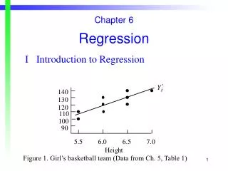
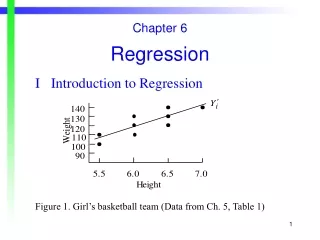
Chapter 6 Regression I Introduction to Regression Figure 1. Girl’s basketball team (Data from Ch. 5, Table 1)
II Criterion for the Line of Best Fit A. Predicting Y from X 2. Line of best fit minimizes the sum of the squared prediction errors
5. Illustration of Y intercept, aY.X, and slope of the best fitting line, bY.X
Table 1. Height and Weight of Girl’s Basketball Team 1 7.0 140 .64 289 13.6 2 6.5 130 .09 49 2.1 3 6.5 140 .09 289 5.1 4 6.5 130 .09 49 2.1 5 6.5 120 .09 9 –0.9 6 6.0 120 .04 9 0.6 7 6.0 130 .04 49 –1.4 8 6.0 110 .04 169 2.6 9 5.5 100 .49 529 16.1 10 5.5 110 .49 169 9.1
1. Predicted weight for girl whose height is Xi = 6.5 C. Predicting X from Y
2. Predicted height for girl whose weight is Yi = 130 D. Comparison of Two Regression Equations
G. Predicted Value of Yi When r = 0 1. Alternative form of the regression equation
III Standard Error of Estimate (SY.X) A. Comparison of SY.X &Standard Deviation (S)
B. Alternative Formula for SY.X 1. Maximum value of SY.X occurs when r = 0 2. Minimum value of SY.X occurs when r = 1
2. Descriptive Application of SY.X Figure 2. Approximately 68.27% of the Y scores fall within Yi ± SY.X
IV Assumptions Associated with Regression and the Standard Error of Estimate A. Regression 1. Relationship between X and Y is linear 2. X and Y are quantitative variables B. Standard Error of Estimate 1. Relationship between X and Y is linear 2. X and Y are quantitative variables 3. Homoscedasticity
V Multiple Regression A. Regression Equation for k Predictors B. Example with n = 5 Subjects and k = 2 Predictors
Table 2. Multiple Regression Example with Two Predictors Observed Predictor Predictor Predicted Prediction Subject Score One Two Score Error __________________________________________________ 1 3 4 3 3.90 -0.90 2 1 2 6 1.02 -0.02 3 2 1 4 1.70 0.30 4 4 6 5 3.75 0.25 5 6 5 1 5.63 0.37 ___________________________________________________
C. Multiple regression equation D. Simple Regression Equations
Table 3. Correlation Matrix for Data in Table 1 ______________________________________ Variable Variable Y X1 X2 ______________________________________ Y 1.000 .777 –.797 X1 1.000 –.338 X2 1.000 ______________________________________
E. Regression Plane for Data in Table 2 Figure 3. (a) Predicted scores fall on the surface of the plane (b) Prediction errors fall above or below the surface of the plane
VI Multiple Correlation (R) A. Multiple Correlation for Data in Table 2
B. Coefficient of Multiple Determination (R2) 1. R2 for the multiple correlation data with two predictors is R2 = (.962)2 = .93 2. Coefficient of determination for the best predictor, X2, is r2 = (–.797)2 = .64 3. Coefficient of determination for the worst predictor, X1, is r2 = (.777)2 = .60 C. The problem of multicollinearity