CHAPTER 5: Regression
CHAPTER 5: Regression. ESSENTIAL STATISTICS Second Edition David S. Moore, William I. Notz, and Michael A. Fligner Lecture Presentation. Chapter 5 Concepts. Regression Lines Least-Squares Regression Line Residuals R-squared r 2 & correlation r Influential Observations.


CHAPTER 5: Regression
E N D
Presentation Transcript
CHAPTER 5:Regression ESSENTIAL STATISTICS Second Edition David S. Moore, William I. Notz, and Michael A. Fligner Lecture Presentation
Chapter 5 Concepts Regression Lines Least-Squares Regression Line Residuals R-squared r2& correlation r Influential Observations
Chapter 5 Objectives Quantify the linear relationship between an explanatory variable (x) and response variable (y). Use a regression line to predict values of (y) for values of (x). Calculate and interpret residuals. Describe cautions about correlation and regression.
Regression Line Example: Predict the number of new adult birds that join the colony based on the percent of adult birds that return to the colony from the previous year. If 60% of adults return, how many new birds are predicted? A regression lineis a straight line that describes how a response variable y changes as an explanatory variable x changes. We can use a regression line to predict the value of y for a given value of x.
Regression Line ^ • x is the value of the independent variable. • “y-hat” is the predicted value of the response variable for a given value of x. • b is the slope, the amount by which y changes for each one-unit increase in x. • ais the intercept, the value of y when x = 0. Regression equation: y = a + bx
Least Squares Regression Line Least Squares Regression Line (LSRL): • The line that minimizes the sum of the squares of the vertical distances of the data points from the line. • Regression equation: y = a + bx • where sx and sy are the standard deviations of the two variables, and r is their correlation. ^ Since we are trying to predict y, we want the regression line to be as close as possible to the data points in the vertical (y) direction.
Facts About Least Squares Regression • Fact 1: The distinction between explanatory and response variables is essential. • Fact 2: The LSRL always passes through (x-bar, y-bar). • Fact 3: The square of the correlation, r2, is an overall measure of the accuracy of a regression. • R-squaredr2is called the coefficient of determination. • R2measure how well your regression equation truly represent your set of data. • R2 indicates the “goodness of fit” of a regression. • R2= 1, it is perfect fit, R2 = 0.5, it is 50% fit.
Prediction via Regression Line • For the returning birds example, the LSRL is y-hat = 31.9343 0.3040x • y-hat is the predicted number of new birds for colonies with x percent of adults returning Suppose we know that an individual colony has 60% returning. What would we predict the number of new birds to be for just that colony? For colonies with 60% returning, we predict the average number of new birds to be: 31.9343 (0.3040)(60) = 13.69 birds
Residuals Gesell Adaptive Score (GAS) and Age at First Word ^ • A residual plotis a scatterplot of the regression residuals against the explanatory variable • used to assess the fit of a regression line • look for a “random” scatter around zero A residualis the difference between an observed value of the response variable and the value predicted by the regression line: residual = y y
Outliers and Influential Points • An outlieris an observation that lies far away from the other observations. • Outliers in the ydirection have large residuals. • Outliers in the x direction are often influential for the least-squares regression line, meaning that the removal of such points would markedly change the equation of the line.
Outliers and Influential Points After removing child 18 From all of the data Gesell Adaptive Score (GAS) and Age at First Word r2 = 11% r2 = 41% Chapter 5
Cautions About Correlation and Regression • Both describe linear relationships. • Both are affected by outliers. • Always plot the data before interpreting. • Beware of extrapolation. • The use of a regression line for prediction outside of the range of values of x uses to obtain the line. Such predictions are often not accurate. • Beware of lurking variables. • These have an important effect on the relationship among the variables in a study, but are not included in the study. • Correlation does not imply causation!
Caution: Beware of Extrapolation Sarah’s height was plotted against her age. Can you predict her height at age 42 months? Can you predict her height at age 30 years (360 months)?
Regression line:y-hat = 71.95 + .383 x Height at age 42 months? y-hat = 88 Height at age 30 years? y-hat = 209.8 She is predicted to be 6’ 10.5” at age 30! Caution: Beware of Extrapolation
Association Does Not Imply Causation • Social Relationships and Health • House, J., Landis, K., and Umberson, D. “Social Relationships and Health,”Science, Vol. 241 (1988), pp 540-545. • Does lack of social relationships cause people to become ill? (there was a strong correlation) • Or, are unhealthy people less likely to establish and maintain social relationships? (reversed relationship) • Or, is there some other factor that predisposes people both to have lower social activity and become ill? • Association not equal to causation in relationship of two variables • Even very strong correlations may not correspond to a real causal relationship (changes in xcausing changes in y). • Correlation sometimes may be explained by a lurking variable
Chapter 5 Objectives Review Quantify the linear relationship between an explanatory variable (x) and response variable (y). Use a regression line to predict values of (y) for values of (x). Calculate and interpret residuals. Describe cautions about correlation and regression.