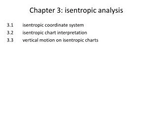
Isentropic Analysis Workshop
Isentropic Analysis Workshop. James T. Moore Saint Louis University. Millersville University Isentropic Workshop: 5 April 2003. Do you know your isentropic geneology?. 2000s??. Theta as a Vertical Coordinate. q = T (1000/P) k , where k = R d / C p Entropy = = C p ln q + const

Isentropic Analysis Workshop
E N D
Presentation Transcript
Isentropic Analysis Workshop James T. Moore Saint Louis University Millersville University Isentropic Workshop: 5 April 2003
Theta as a Vertical Coordinate • q= T (1000/P)k, where k= Rd / Cp • Entropy = = Cp lnq + const • If = const then q = const, so constant entropy sfc = isentropic sfc • Three types of stability, since dq/ dz = (q/T) [d - ] • stable: < d, q increases with height • neutral: = d, q is constant with height • unstable: > d, q decreases with height • So, isentropic surfaces are closer together in the vertical in stable air and further apart in less stable air.
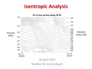
Visualizing Static Stability – Vertical Gradients of Vertical changes of potential temperature related to lapse rates: U = unstable N = neutral S = stable VS = very stable
Theta as a Vertical Coordinate • Isentropes slope DOWN toward warm air, UP toward cold air – this is opposite to the slope of pressure surfaces: since q= T (1000/P)k, as P increases (decreases), T increases (decreases) to keep constant (as on a skew-T diagram). • Isentropes slope much greater than pressure surfaces given the same thermal gradient; as much as one order of magnitude more! • On an isentropic surface an isotherm = an isobar = an isopycnic (const density); (remember: P = RdT) • On an isentropic surface we analyze the Montgomery streamfunction to depict geostrophic flow, where: M = y = Cp T + gZ ;
Isentropic Analysis: Advantages • For synoptic scale motions, in the absence of diabatic processes, isentropic surfaces are material surfaces, i.e., parcels are thermodynamical bound to the surface • Horizontal flow along an isentropic surface contains the adiabatic component of vertical motion often neglected in a Z or P reference system • Moisture transport on an isentropic surface is three-dimensional - patterns are more spatially and temporally coherent than on pressure surfaces • Isentropic surfaces tend to run parallel to frontal zones making the variation of basic quantities (u,v, T, q) more gradual along them.
Plan view of an isentropic surface analysis Blue dashed lines = isobars, red dashed lines are isohumes
Moisture transport and lift along an isentropic surface 6 8 Isentropicmountain Warm moist air
Advection of Moisture on an Isentropic Surface Moist air from low levels on the left (south) is transported upward and to the right (north) along the isentropic surface. However, in pressure coordinates water vapor appears on the constant pressure surface labeled p in the absence of advection along the pressure surface --it appears to come from nowhere as it emerges from another pressure surface. (adapted from Bluestein, vol. I, 1992, p. 23)
Isentropic Analysis: Advantages • Atmospheric variables tend to be better correlated along an isentropic surface upstream/downstream, than on a constant pressure surface, especially in advective flow • The vertical spacing between isentropic surfaces is a measure of the dry static stability. Convergence (divergence) between two isentropic surfaces decreases (increases) the static stability in the layer. • The slope of an isentropic surface (or pressure gradient along it) is directly related to the thermal wind. • Parcel trajectories can easily be computed on an isentropic surface. Lagrangian (parcel) vertical motion fields are better correlated to satellite imagery than Eulerian (instantaneous) vertical motion fields.
Cross section for 00 UTC 17 April 1976 from Winslow, AZ to Tucson, AZ to Fraccionamiento, MX. Solid lines are isentropes and dashed lines are isotachs (m s-1). (Shapiro 1981, JAS) J Note how the isentropes run parallel to the frontal zone – NOT across it; also note the strong vertical wind shear
Station Model for Isentropic Analysis Montgomery Streamfunction (J kg-1) Pressure (mb) 785 29460 10 85 Static Stability over 8 K layer (4 K below and 4 K above) in mb Mixing Ratio (gm kg-1) Wind Direction and Speed (knots)
Choosing the “Right” Isentropic Surface(s) • The “best” isentropic surface to diagnose low-level moisture and vertical motion varies with latitude, season, and the synoptic situation. There are various approaches to choosing the “best” surface(s): • Use the ranges suggested by Namias (1940) : • SeasonLow-Level Isentropic Surface • Winter 290-295 K • Spring 295-300 K • Summer 310-315 K • Fall 300-305 K
Choosing the “Right” Isentropic Surface(s) BEST METHOD: • Compute a cross section of isentropes and isohumes ( mixing ratios) normal to a jet streak or baroclinic zone in the area of interest. • Choose the low-level isentropic surface that is in the moist layer, displays the greatest slope, and stays 50-100 hPa above the surface. • A rule of thumb is to choose an isentropic surface that is located at ~700-750 hPa above your area (as with the “Garcia” method for forecasting snowfall)
Using an Isentropic Cross Section to Choose a Surface: Isentropic Cross Section for 00 UTC 05 Dec 1999
Isentropic Moisture Parameters • Lifting Condensation Pressure (LCP): The pressure to which a parcel of air must be raised dry-adiabatically in order to reach condensation. Represents moisture differences better than mixing ratio at low values of mixing ratio. Condensation pressure on an isentropic surface is equivalent to dew point on a constant pressure surface. • Condensation Difference (CD):The difference between the actual pressure and the condensation pressure for a point on a isentropic surface. The smaller the condensation difference, the closer the point is to saturation. Due to smoothing and round off errors, a difference < 20 hPa represents saturation. Values < 100 hPa indicated near saturation. Condensation difference on an isentropic surface is equivalent to dew point depression on a constant pressure surface.
Isentropic Moisture Parameters Moisture Transport Vectors (MTV): • Defined as the product of the horizontal velocity vector, V, and the mixing ratio, q. Units are gm-m/kg-s ; values typically range from 50-250, depending upon the level and the season. • Typically, stable precipitation due to isentropic upglide falls downstream from the maximum of the moisture transport vector magnitude in the northern gradient region. The moisture transport vectors and isopleths of the magnitude of the moisture transport vectors are usually displayed. • Note that the negative divergence of the MTVs is equal to the horizontal moisture convergence, since
Isentropic Analysis: Disadvantages • The temporal continuity of isentropic surfaces are disrupted by diabatic heating/cooling; diabatic heating (cooling) causes isentropic surfaces to move downward (upward) • Isentropic surfaces are vertical in regions of neutral lapse rates (i.e., = d) and “fold” in regions of superadiabatic lapse rates (i.e., > d) • Forecaster must choose 1-2 isentropic surfaces to analyze in lower troposphere, not pre-selected like pressure surfaces. • Construct an isentropic cross section along with isohumes normal to the baroclinic zone and choose an isentropic surface – but stay out of that nasty boundary layer!
Neutral-Superadiabatic Lapse Rates SA=superadiabatic and N=neutral
Vertical Resolution is a Function of Static Stability LS = less stable (weak static stability) and VS = very stable (strong static stability)
Radiational Heating/Cooling Disrupts the Continuity of Isentropic Surfaces As time increases solar heating causes the 300 K isentropic surface to become “redefined” at higher pressures Namias, 1940: An Introduction to the Study of Air Mass and Isentropic Analysis, AMS, Boston, MA.
304 K Isentropic Surface for 00 UTC 3 May 2002 Note loss of data in SE U.S. and in Texas…304 K surface went underground
Computing Vertical Motion A B C Term A: local pressure change on the isentropic surface Term B: advection of pressure on the isentropic surface Term C: diabatic heating/cooling term (modulated by the dry static stability. Typically, at the synoptic scale it is assumed that terms A and C are nearly equal in magnitude and opposite in sign.
Example of Computing Vertical Motion 1. Assume isentropic surface descends as it is warmed by latent heating (local pressure tendency term): P/ t = 650 – 550 hPa / 12 h = +2.3 bars s-1 (descent) 2. Assume 50 knot wind is blowing normal to the isobars from high to low pressure (advection term): V P = (25 m s-1) x (50 hPa/300 km) x cos 180 V P = -4.2 bars s-1 (ascent) 3. Assume 7 K diabatic heating in 12 h in a layer where increases 4 K over 50 hPa (diabatic heating/cooling term): (d/dt)(P/ ) = (7 K/12 h)(-50 hPa/4K) = -2 bars s-1 (ascent)
Local pressure tendency term computed over 12, 6 and 3 hours by Homan and Uccellini, 1987 (WAF, vol. 2, 206-228)
Isentropic System-Relative Vertical Motion Define Lagrangian; no - diabatic heating/cooling System tendency Assume tendency following system is = 0; e.g., no deepening or filling of system with time. Insert pressure, P, as the variable in the ( )
System-Relative Isentropic Vertical Motion • Defined as: • ~ (V – C) P Where = system-relative vertical motion in bars sec-1 V= wind velocity on the isentropic surface C = system velocity, and • P = pressure gradient on the isentropic surface C is computed by tracking the associated vorticity maximum on the isentropic surface over the last 6 or 12 hours (one possible method); another method would be to track the motion of a short-wave trough on the isentropic surface
System-Relative Isentropic Vertical Motion Including C, the speed of the system, is important when: * the system is moving quickly and/or * a significant component of the system motion is across the isobars on an isentropic surface, e.g., if the system motion is from SW-NE and the isobars are oriented N-S with lower pressure to the west, subtracting C from V is equivalent to “adding” a NE wind, thereby increasing the isentropic upslope.
When is C important to use when computing isentropic omegas? Vort Max at t1 In regions of isentropic upglide, this system-rela- tive motion vector, C, will enhance the uplift (since C is subtracted from the Velocity vector), Vort Max at to
Computing Isentropic Omegas • Essentially there are three approaches to computing isentropic omegas: • Ground-Relative Method (V P) : • Okay for slow-moving systems (P/ t term is small) • Assumes that the advection term dominates (not always a good assumption) • System-Relative Method ( (V-C) P ) : • Good for situations in which the system is not deepening or filling rapidly • Also useful when the time step between map times is large (e.g., greater than 3 hours) • S-R velocity vectors are useful in computing S-R MTVs • Brute-Force Computational Method ( P/ t + V P ): • Best for situations in which the system is rapidly deepening or filling • Good approximation when data are available at 3 h or less interval, allowing for good estimation of local time tendency of pressure
Three-Dimensional Isentropic Topography cold warm
Thermal Wind Relationship in Isentropic Coordinates • Usually only the wind component normal to the plane of the cross section is plotted; positive (negative) values indicate wind components into (out of) the plane of the cross section. • With north to the left and south to the right: • when isentropes slope down, the thermal wind is into the paper, i.e, the wind component into the cross-sectional plane increases with height • when isentropes slope up, the thermal wind is negative, i.e., the wind component out of the cross-sectional plane increases with height.
Thermal Wind Relationship in Isentropic Coordinates • Isentropic surfaces have a steep slope in regions of strong • baroclinicity. Flat isentropes indicate barotropic conditions • and little/no change of the wind with height. • Frontal zones are characterized by sloping isentropic surfaces which are vertically compacted (indicating strong static stability). • In the stratosphere the static stability increases by about one order of magnitude.
250 mb Winds and Isotachs from Eta 24 h fcst valid 00 29 Nov 2001
Cross section of and normal wind components; dashed (solid) yellow = out of (into) the cross-sectional plane. 24 h Eta forecast valid 00 UTC 29 November 2001
The “Garcia Method”: Forecasting Snowfall Using Mixing Ratios on an Isentropic Surface • Determine the geographic location (area of concern) for the expected snowfall. • Determine what isentropic surface best intersects the 700-750 mb layer over the area of concern. • Analyze pressure every 50 mb and mixing ratios every 1 g kg-1. • Determine the mixing ratio value over the area of concern and from the isentropic wind field approximate the mixing ratio to be advected into the are during the next 12 h. From these two values calculate an average mixing ratio for the 12 h period.
The “Garcia Method” (cont.) • Determine if the dynamic forcing for lift necessary for maximum snowfall will exist for most or just part of the 12 h period. This is a subjective “call” based upon experience, observations, and model guidance. • Empirical observations have shown that a 2:1 ratio relationship exists between the maximum snowfall amount and the average mixing ratio. For example, for an average mixing ratio of 3 g kg-1 you would expect about 6 inches for the maximum snowfall. For the Garcia method and update see the following website: www.crh.noaa.gov/techpapers/memos/TM-116/TM-116.html
The “Garcia Method” -- Update • Garcia amended his original method to account for: • Heavy snowfall events in which the snow:liquid equivalent ratio, in very cold and dry Arctic air, has to be taken into account. Snow:liquid equivalent ratios in these cases can be as high as 30:1. • Heavy snowfall events in which snowfall was enhanced due to jet streaks or coupled jet streaks. In these cases thundersnow is often observed due to upright or slantwise convection. Garcia recommends a 4:1 ratio for snowfall:mixing ratio. Of course, the speed of these dynamic systems must be taken into account as well.
11 March 2000 Case Study • A late-winter, surprise heavy snow event occurred during the morning of 11 March 2000. Forecasters anticipated 1-2 inches of snow, but the system became convective, resulting in heavy snow in a narrow band in Missouri and Illinois. • Snowfall occurred mainly during the morning hours (0900—1500 UTC) in east-central Missouri. • “Thundersnow” was observed at Spirit of St. Louis (KSUS) and St. Louis International (KSTL) airports for approximately 2 hours, beginning shortly after 1200 UTC.
Storm Total Snowfall 11 March 2000 Total snowfall in Missouri and Illinois in inches, as analyzed by F. H. Glass of KSTL NWSFO.
Water Vapor Satellite LoopValid 0015-0315 UTC; 0715-2315 UTC
0000 UTC 11 March 2000 Surface Analysis 0000 UTC surface analysis. Blue scalloped line denotes region reporting snow.
0600 UTC 11 March 2000 Surface Analysis 0600 UTC surface analysis. Blue scalloped line denotes region reporting snow.
1200 UTC 11 March 2000 Surface Analysis 1200 UTC surface analysis. Blue scalloped line denotes region reporting snow.
1800 UTC 11 March 2000 Surface Analysis 1800 UTC surface analysis. Blue scalloped line denotes region reporting snow.