Chapter II Isentropic Flow
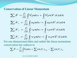
Conservation of Linear Momentum For one dimensional inlets and outlets the linear momentum conservation law reduces to .

Chapter II Isentropic Flow
E N D
Presentation Transcript
Conservation of Linear MomentumFor one dimensional inlets and outlets the linear momentum conservation law reduces to Prof. Dr. MOHSEN OSMAN
The Angular – Momentum TheoremA control volume analysis can be applied to the angular-momentum relation by letting our dummy variable B be the angular – momentum vector . If o is the point about which moments are desired; the angular momentum about o is given by:elemental mass position vector X velocity of that element The amount of angular momentum per unit mass is seen to be: The Reynolds’ transport theorem then tells us thatConservation of Angular Momentum Prof. Dr. MOHSEN OSMAN
For fixed control-volume If there are only one-dimensional inlets and exits, the angular – momentum flux terms evaluated on the control surface becomeExample # 3The sketch shows a vane with a turning angle β which moves with a steady speed U. The vane receives a jet which leaves a fixed nozzle with speed V. (a) Assuming that the vane is mounted on rails as shown in the sketch, show that the work done against the restraining force is a maximum when (b) Assuming that there are a large number of such vanes attached to be rotating wheel moving with peripheral speed U, show that the work delivered to the wheel is a maximum when Prof. Dr. MOHSEN OSMAN
(a) Apply conservation of linear momentum equation: Since then, or Apply conservation of linear momentum equation in the x-direction Substitute for then, Multiply the equation by -1 Since Power = F x Vvane OR then, For maximum , differentiate w.r.t. U and equate to zero; Prof. Dr. MOHSEN OSMAN
V = U refused then, V = 3U OR for maximum work against (b) For a large number of such vanes attached to a rotating wheel moving with peripheral speed U, the mass flow rateApply the conservation of angular momentum equation: Since Differentiate w.r.t. U and equate to zero: Prof. Dr. MOHSEN OSMAN
The Energy EquationAs our fourth and final basic law we apply the Reynolds’ transport theorem to the first law of thermodynamics,The dummy variable B becomes energy E , and the energy per unit mass is The first law of thermodynamics can then be written for a fixed control volume as followsThe system energy per unit mass e may be of several types:where could encompass chemical reactions, nuclear reactions, and electrostatic or magnetic field effects. Prof. Dr. MOHSEN OSMAN
We neglect here and consider only the first three terms:Using for convenience the over dot to denote the time derivative, we shall divide the work term into three partsThe pressure work equals the pressure force on a small surface element dA times the normal velocity component into the control volume. The total pressure work is the integral over the control surfaceFinally, the shear work due to viscous stresses occurs at the control surface consists of each viscous stress (one normal and two tangential) and the respective velocity component Prof. Dr. MOHSEN OSMAN
Whereis the stress vector on the elemental surface dA. This term may vanish or be negligible according to the particular type of surface at that part of the control volume (C.V).Solid SurfaceFor all parts of the control surface which are solid confining walls, from the viscous no-slip condition; hence identically.Surface of a MachineHere the viscous work is contributed by the machine, and so we absorb this work in the term .An Inlet or OutletAt an inlet or outlet, the flow is approximately normal to the element dA; hence the only viscous-work term comes from the normal stress . Prof. Dr. MOHSEN OSMAN
Since viscous normal stresses are extremely small in all but rare cases, it is customary to neglect viscous work at inlets and outlets of the control volume.Streamline SurfaceIf the control surface is a streamline such as the upper curve in the boundary-layer analysis, the viscous-work term must be evaluated and retained if shear stresses are significant along this line. In the particular case of streamline outside the boundary-layer, the viscous work is negligible.The net result of the above discussion is that the rate-of-work term in the energy equation consists essentially of ss = stream surface Prof. Dr. MOHSEN OSMAN
The control-volume energy equation thus becomesUsing , we see that the enthalpy occurs in the control surface integral. The final general form for the energy equation for a fixed control volume becomes: One–Dimensional Energy–Flux TermsIf the control volume has a series of one-dimensional inlets and outlets, the surface integral reduces to a summation of outlet fluxes minus inlet fluxes Prof. Dr. MOHSEN OSMAN
Where values of and are taken to be averages over each cross section.The Steady–Flow Energy EquationFor steady flow with one inlet and one outlet, both assumed one–dimensional, the energy equation reduces to a celebrated relation used in many engineering analyses. Let section 1 be the inlet and section 2 be the outlet, thenBut, from continuity, and we can rearrange the energy equation as follows:Stagnation Enthalpy Stagnation Enthalpy Prof. Dr. MOHSEN OSMAN
Chapter IIIsentropic Flow General Features of Isentropic Flow The flow in pipes and ducts is very often adiabatic. When the duct is short, as it is in nozzles, diffusers, the frictional effects are comparatively small, and the flow may as a first approximat –ion be considered reversible, and, therefore isentropic. The one – dimensional approximation A one – dimensional flow is a flow in which the rate of change of fluid properties normal to the streamline direction is negligibly small compared with the rate of charge along the streamline. If the properties vary over each cross section and we are applying the one – dimensional assumption to the flow in ducts, we in effect deal with certain kinds of average properties for each cross section. Prof. Dr. MOHSEN OSMAN
Consider the isentropic flow of any fluid through a passage of vary- ing cross section. The following physical equations may be written for a control surface extending between the stagnation section and any other section in the channel;I – The first law of Thermodynamics (steady-flow energy equation)Or = stagnation enthalpyThis is hold for steady adiabatic flow of any compressible fluid outside the boundary layer. For perfect gases : & From the first law of Thermodynamics : Prof. Dr. MOHSEN OSMAN