Finite Domains
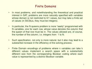
Finite Domains. In most problems, and notwithstanding the theoretical and practical interest in SAT, problems are more naturally specified with variables whose domain is not restricted to 0/1 values, but may take a finite set of values (in SICStus, they must be integers).

Finite Domains
E N D
Presentation Transcript
Finite Domains • In most problems, and notwithstanding the theoretical and practical interest in SAT, problems are more naturally specified with variables whose domain is not restricted to 0/1 values, but may take a finite set of values (in SICStus, they must be integers). • In particular, the N queens problem is more “easily” programmed with N variables, one for each row, whose value denotes the column that the queen of that row must be in. The values allowed are, of course, the number of the column, i.e. integers from 1 to N. • Such specification, not only is more natural, but it also may lead to a substantial increase in the efficiency of the solving process. • Finite Domain encodings of problems where n variables can take k different values implement a search space with a substantially different size from the corresponding Boolean coding where each value is represented by a distinct Boolean variable.
Finite Domains • To compare the search spaces of Boolean and Finite Domain encodings for problems where n variables can take k different values we note that: • Boolean Encodings - k*n boolean variables ( 0/1). Search Space = 2kn. • Finite Domains - n variables each with k possible values Search Space = kn • Ratio of the Search Spaces r= 2kn / 2log2k*n = 2 (k-log2(k))*n For example, in the N-queens problem, we have • N = 8 k= 8, and r=2(8-3)*8 = 240 1012 • N = 16 k=16, and r=2(16-4)*16 = 2192 1058
Finite Domains • Of course, the ratio of the search spaces that are actually searched is not so large, namely due to constraint propagation. • For example, in the N-queens problem, since only one queen may be placed in each row (and column), the boolean code will have exclusivity constraints of the type at_most_one([B1, B2, ...Bk]), for queens in the same row or column. • Efficient Boolean propagation imposes a 0 value to all the other variables, when one of the set takes value 1. • Still, the differences may be significant, as can be seen in the programs coded directly in finite domains • queens_sat_bk and queens_sat_fd • queens_bk and queens_fd
Finite Domains • The efficiency of the CLP programs over finite domains (including the Boolean case) may still be improved by making use of • Adequate Propagation Algorithms • Appropriate Heuristics for selection of the • Variable to label • Value to assign • These variations may be found in program queens_fd_xc where a number of possibilities are parameterised.
Finite Domains • The changes in efficiency in the various programs of the N queens problem were due to different • Propagation Algorithms • Heuristics for Variable Selection • Before investigating these issues, namely the Propagation Algorithms, we should formalise a number of concepts that will be used • Constraints and Constraint Network • Partial and Total Solutions • Satisfaction and Consistency
Basic Definitions - Domain Definition (Domain of a Variable): • The domain of a variable is the (finite) set of values that can be assigned to that variable. • Given some variable X, its domain will be usually referred to as dom(X) or, simply, Dx. • Example: The N queens problem may be modelled by means of N variables, X1 to Xn, all with the domain from 1 to n. Dom(Xi) = {1,2, ..., n} or Xi :: 1..n.
Basic Definitions - Labels • To formalise the notion of the state of a variable (i.e. its assignment with one of the values in its domain) we have the following Definition (Label): • A label is a Variable-Value pair, where the Value is one of the elements of the domain of the Variable. • The notion of a partial solution, in which some of the variables of the problem have already assigned values, is captured by the following Definition (Compound Label): • A compound label is a set of labels with distinct variables.
Basic Definitions - Constraint • We come now to the formal definition of a constraint Definition (Constraint): • Given a set of variables, a constraint is a set of compound labels on these variables. • Alternatively, a constraint may be defined simply as a relation, i.e. a subset of the cartesian product of the domains of the variables involved in that constraint. • For example, given a constraint Rijk involving variables Xi, Xj and Xk, then Rijk dom(Xi) x dom(Xj) x dom(Xk)
Basic Definitions - Constraint • Given a constraint C, the set of variables involved in that constraint is denoted by vars(C). • Simetrically, the set of constraints in which variable X participates is denoted by cons(X). • Notice that a constraint is a relation, not a function, so that it is always Cij = Cji. • In practice, constraints may be specified by • Extension: through an explicit enumeration of the allowed compound labels; • Intension: through some predicate (or procedure) that determines the allowed compound labels.
Basic Definitions – Constraint Definition • For example, the constraint C13 involving X1 and X3 in the 4-queens problem, may be specified • By extension (label form): C13 = {{X1-1,X3-2},{X1-1,X3-4},{X1-2,X3-1},{X1-2,X3-3}, {X1-3,X3-2},{X1-3,X3-4},{X1-4,X3-1},{X1-4,X3-3}}. or, in tuple (relational) form, omitting the variables C13 = {<1,2>,<1,4>,<2,1>,<2,3>,<3,2>,<3,4>,<4,1>,<4,3>}. • By intension: C13 = (X1 X3) (1+X1 3+X3) (3+X1 1+X3).
Basic Definitions – Constraint Arity Definition (Constraint Arity): • The constraint arity of some constraint C is the number of variables over which the constraint is defined, i.e. the cardinality of the set Vars(C). • Despite the fact that constraints may have an arbitrary arity, an important subset of the constraints is the set of binary constraints. • The importance of such constraints is two fold • All constraints may be converted into binary constraints • A number of concepts and algorithms are appropriate for these constraints.
Basic Definitions – Binary Constraints Conversion to Binary Constraints • An n-ary constraint, C, defined by k compound labels on its variables X1 to Xn, is equivalent to n binary constraints, C0i, through the addition of a new variable, X0, whose domain is the set 1 to k. In practice, • The k n-ary labels may be sorted in some arbitrary order. • Each of the n binary constraints C0i relates the new variable X0 with the variable Xi. • The compound label {Xi-vi, X0-j} belongs to constraint C0i iff Xi-vi belongs to the j-th compound label that defines C.
Basic Definitions – Binary Constraints Example: Given variables X1 to X3, with domains 1 to 3, the following ternary constraint C is composed of 6 labels.. C(X1, X2, X3) = {<1,2,3>,<1,3,2>,<2,1,3>,<2,3,1> ,<3,1,2>,<3,2,1>} Each of the labels may be associated to a value from 1 to 6 1 : <1,2,3>, 2 : <1,3,2>, ... , 6: <3,2,1> Now, the following binary constraints, C01 to C03, are equivalent to the initial ternary constraint C C01(X0, X1) = {<1,1>, <2,1>, <3,2>, <4,2>, <5,3>, <6,3>} C02(X0, X2) = {<1,2>, <2,3>, <3,1>, <4,3>, <5,1>, <6,2>} C03(X0, X3) = {<1,3>, <2,2>, <3,3>, <4,1>, <5,2>, <6,1>}
Basic Definitions –Constraint Satisfaction Definition (Constraint Satisfaction 1): • A compound label satisfies a constraint if their variables are the same and if the compound label is a member of the constraint. • In practice, it is convenient to generalise constraint satisfaction to compound labels that strictly contain the constraint variables. Definition (Constraint Satisfaction 2): • A compound label satisfies a constraint if its variables contain the constraint variables and the projection of the compound label to these variables is a member of the constraint.
Basic Definitions –Constraint Satisfaction Problem Definition (Constraint Satisfaction Problem): • A constraint satisfaction problem is a triple <V, D, C> where • V is the set of variables of the problem • D is the domain(s) of its variables • C is the set of constraints of the problem Definition (Problem Solution): • A solution to a Constraint Satisfaction Problem P, defined as the tuple <V, D, C>, is a compound label over the variables V of the problem, which satisfies all the constraints in C.
Basic Definitions – Constraint Graph • For convenience, the constraints of a problem may be considered as forming a special graph. Definition (Constraint Graph or Network): • The Constraint Graph or Network of a binary constraint satisfaction problem is defined as follows • There is a node for each of the variables of the problem. • For each non-trivial constraint of the problem, involving one or two variables, the graph contains an arc linking the corresponding nodes. • When the problems include constraints with arbitrary arity, the Constraint Network may be formed after converting these constraints on its binary equivalent.
Basic Definitions – Constraint Hiper-Graph • When it is not convenient for some reason to convert constraints to their binary equivalent, the problem may be represented by an hiper-graph. Definition (Constraint Hyper-Graph): • Any constraint satisfaction problem with arbitrary n-ary constraints may be represented by a Constraints Hiper-Graph formed as follows: • There is a node for each of the variables of the problem. • For each constraint of the problem, the graph contains an hiper-arc linking the corresponding nodes. • Of course, when the problem has only binary constraints, the hiper-graph degenerates into the simpler graph.
X1 in 1..4 C12 C13 R14 R23 X2 in 1..4 X3 in 1..4 C34 C24 X4 in 1..4 Example: 4 - Queens Example: The 4 queens problem may be specified by the following constraint network: <1,2>, <1,4>, <2,1>, <2,3>, <3,2>, <3,4>, <4,1>, <4,3>
Basic Definitions – Graph Density Definition (Complete Constraint Network): • A constraint netwok is complete, when there is an arc connecting any two nodes of the graph (i.e. when there is a constraint over any pair of variables). • The 4 queens problem (in fact, any n queens problem) has a complete graph. • However, this is often not the case: most graphs are sparse. In this case, it is important to measure the density of the constraint network. • Definition (Density of a Constraint Graph): • The density of a constraint graph is the ratio between the number of its arcs and the number of arcs of a complete graph on the same number of nodes
Basic Definitions – Problem Difficulty • In principle, the “difficulty” of a constraint problem is related to the density of its graph. • Intuitively, the denser the graph is, the more difficult the problem becomes, since there are more opportunities to invalidate a compound label. • It is important to distinguish between the difficulty of a problem and the difficulty of solving the problem. • In particular, a difficult problem may be so difficult that it is trivial to find it to be impossible! • The “difficulty” of a problem is also related to the difficulty of satisfying each of its constraints. Such difficulty may be measured through its “tightness”.
Basic Definitions – Constraint Tightness Definition (Tightness of a Constraint): • Given a constraint C on variables X1 ... Xn, with domains D1 to Dn, the tightness of C is defined as the ratio between the number of labels that define the constraint and the size (i.e. the cardinality) of the cartesian product D1 x D2 x .. Dn. • For example, the tightness of constraint C13 of the 4 queens problem, on variables X1 and X3 with domains 1..4 C13 = {<1,2>, <1,4>, <2,1>, <2,3>, <3,2>, <3,4>, <4,1>, <4,3>} is 1/2, since there are 8 tuples in the relation out of the possible 16 (4*4). • The notion of tightness may be generalised for the whole problem.
Basic Definitions – Problem Tightness • Definition (Tightness of a Problem): • The tightness of a constraint satisfaction problem with variables X1 ... Xn, is the ratio between the number of its solutions and the cardinality of the cartesian product D1 x D2 x .. Dn. • For example, the 4 queens problem, that has only two solutions <2,4,1,3> e <3,1,4,2> has tightness 2/(4*4*4*4) = 1/128.
Basic Definitions – Constraint Tightness • The difficulty in solving a constraint satisfaction problem is related both with the • The density of its graph and • Its tightness. • As such, when testing algorithms to solve this type of problems, it is usual to generate random problem instances, parameterised not only by the number of variables and the size of their domains, but also by the density of its graph and the tightness of its constraints. • The study of these issues has led to the conclusion that constraint satisfaction problems often exhibit a phase transition, which should be taken into account in the study of the algorithms. • This phase transition typically contains the most difficult instances of the problem, and separates the instances that are trivially satisfied from those that are trivially insatisfiable.
difficulty 4.3 # clauses / # variables Basic Definitions – Phase Transition in SAT • For example, in SAT, it has been found that the phase transition occurs when the ration of clauses to variables is around 4.3.
Basic Definitions – Redundancy • Another issue to consider in the difficulty of solving a constraint satisfaction problem is the potential existence of redundant values and labels in its constraints. Definition (Redundant Value): • A value in the domain of a variable is redundant, if it does not appear in any solution of the problem. Definition (Redundant Label): • A compound label of a constraint is redundant if it is not the projection to the constraint variables of a solution to the whole problem. • Redundant values and labels increase the search space useless, and should thus be avoided. There is no point in testing a value that does not appear in any solution !
Basic Definitions – Redundancy Example: The 4 queens problem only admits two solutions: <2,4,1,3> and <3,1,4,2>. • Hence, values 1 and 4 are redundant in the domain of variables X1 and X4, and values 2 and 3 are redundant in the domain of variables X2 and X3. • Regarding redundant labels, labels <2,3> and <3,2> are redundant in constraint C13.
X1 in 1,2,3,4 C12 C13 R14 R23 X2 in 1,2,3,4 X3 in 1,2,3,4 C34 C24 X4 in 1,2,3,4 Basic Definitions – Redundancy Example: The 4 queens problem, which only admits the two solutions <2,4,1,3> e <3,1,4,2> may be “simplified” by elimination of the redundant values and labels. {<1,2>, <1,4>, <2,1>, <2,3>, <3,2>, <3,4>, <4,1>, <4,3>}
Basic Definitions – Equivalent Problems • Of course, any problem should be equivalent to any of its simplified versions. Formally, Definition (Equivalent Problems): • Two problems P1 = <V1, D1, C1> and P2 = <V2, D2, C2> are equivalent iff they have the same variables (i.e. V1 = V2) and the same set of solutions. • The “simplification” of a problem may also be formalised Definition (Reduced Problem): • A problem P=<V,D,C> is reduced to P’=<V’, D’, C’> if • P e P’ are equivalent; • The domains D’ are included in D; and • The constraints C’ are at least as restrictive as those in C.
Constraint Solving Methods • As shown before, and independently of any problem reduction, a generate and test procedure to solve a Constraint Satisfaction Problem is usually very inneficient. • Nevertheless, this is the approach taken in local search methods (simulated annealing or genetic algorithms) – although mostly in an optimisation context ! • It is thus often preferable to use a solving method that is constructive and incremental, whereby a compound label is being completed (constructive), one variable at a time (incremental), until a solution is reached. • However, one must check that at every step in the construction of a solution the resulting label has still the potential to reach a complete solution.
Constraint Solving Methods • Ideally, a compound label should be the projection of some problem solution. • Unfortunately, in the process of solving a problem, its solutions are not known yet! • Hence, one may use a notion weaker than that of a (complete) solution, namely Definition (k-Partial Solution): • A k-partial solution of a constraint solving problem P, defined as P = <V,D,C>, is a compound label on a subset of k of its variables, Vk, that satisfies all the constraints in C whose variables are included in Vk.
1 4 2 3 4 1 1 4 3 2 Constructive Solving Methods • This is of course, the basis of the solving methods that use some form of backtracking. If conveniently performed, backtracking may be regarded as a tree search, where the partial solutions correspond to the internal nodes of the tree and complete solutions to its leaves.
Problem Search Space • Clearly, the more a problem is reduced, the easier it is, in principle, to solve it. • Given a problem P=<V,D,C> with n variables X1,..,Xn the potential search space where solutions can be found (i.e. the leaves of the search tree with compound labels {<X1-v1>, ..., <Xn-vn>}) has cardinality #S = #D1 * #D2 * ... * #Dn • Assuming identical cardinality (or some kind of average of the domains size) for all the variable domains, (#Di = d) the search space has cardinality #S = dn which is exponential on the “size” n of the problem.
Reduction of the Search Space • If instead of the cardinality d of the initial problem, one solves a reduced problem whose domains have lower cardinality d’ (<d) the size of the potential search space also decreases exponentially! S’/S = d’n / dn = (d’/d)n • Such exponential decreases may be very significant for “reasonably” large values of n, as shown in the table.
Reduction of the Search Space • In practice, this potential narrowing of the search space has a cost involved in finding the redundant values (and labels). • A detailed analysis of the costs and benefits in the general case is extremely complex, since the process depends highly on the instances of the problem to be solved. • However, it is reasonable to assume that the computational effort spent on problem reduction is not proportional to the reduction achieved, becoming less and less efficient. • After some point, the gain obtained by the reduction of the search space does not compensate the extra effort required to achieve such reduction. .
Effort spent in solving the problem Computational Cost R+S Combined Cost R - Reduction Cost S- Search Cost Amount of Reduction Achieved Reduction of the Search Space Qualitatively, this process may be represented by means of the following graph
Reduction of the Search Space • The effort in reducing the domains must be considered within the general scheme to solve the problem. • In Constraint Logic Programming, the specification of the constraints usually precedes the enumeration of the variables. Problem(Vars):- Declaration of Variables and Domains, Specification of Constraints, Labelling of the Variables. • However, the execution model alternates enumeration with propagation, making it possible to reduce the problem at various stages of the solving process.
Reduction of the Search Space • Given a problem with n variables X1 a Xn the execuction model follows the following pattern: Declaration of Variables and Domains, Specification of Constraints, indomain(X1), % value selection with backtraking propagation, % reduction of problem X2 to Xn indomain(X2), propagation, % reduction of problem X3 to Xn ... indomain(Xn-1) propagation, % reduction of problem Xn indomain(Xn)
Domain Reduction – Consistency Criteria • Once formally defined the notion of problem reduction, one must discuss the actual procedure that may be used to achieve it. • First of all, one must ensure that whatever procedure is used, the reduction keeps the problem equivalent to the initial one. • Here we have a small problem, since the definition of equivalence requires the solutions to be the same and we do not know in general what the solutions are! • Nevertheless, the solutions will be the same if in the process of reduction we have the guarantee that “no solutions are lost”. Such guarantees are met by several criteria.
Domain Reduction – Consistency Criteria • Consistency criteria enable to establish redundant values in the variables domains in an indirect form, i.e. requiring no prior knowledge on the set of problem solutions. • Hence, procedures that maintain these criteria during the “propagation” phases, will eliminate redundant values and so decrease the search space on the variables yet to be enumerated. • In constraint satisfaction problems with binary constraints, the most usual criteria are, in increasingly complexity order, • Node Consistency • Arc Consistency • Path Consistency
Domain Reduction – Node Consistency Definition (Node Consistency): • A constraint satisfaction problem is node-consistent if no value on the domain of its variables violates the unary constraints. • This criterion may seem both obvious and useless. After all, who would specify a domain that violates the unary constraints ?! • However, this criterion must be regarded within the context of the execution model that incrementally completes partial solutions. Constraints that were not unary in the initial problem become so when one (or more) variables are enumerated.
X1 in 1..4 C12 R13 R14 C23 X2 in 1..4 X3 in 1..4 X2 1,2 X3 1,3 C34 C24 X4 in 1..4 C23 X2 in 1..4 X3 in 1..4 X4 1,4 C34 C24 X4 in 1..4 Domain Reduction – Node Consistency Example: • After the initial launching of the constraints, the constraint network model in the left models the 4 queens problem. • After enumeration of the variable X1, i.e. X1=1, constraints C12, C13 and C14 become unary !!
X2 1,2 X3 1,3 X4 1,4 C23 X2 in 3,4 X3 in 2,4 X2 1,2 X3 1,3 C34 C24 X4 1,4 X4 in 2,3 Domain Reduction – Node Consistency • An algorith that maintains node consistency should remove from the domains of the “future” variables the appropriate values. • Maintaining node consistency achieves a domain reduction similar to what was achieved in propagation with the boolean formulation.
Maintaining Node Consistency • Given the simplicity of the node consistency criterion, an algorithm to maintain it is very simple and with low complexity. • A possible algorithm is NC-1, below. procedure NC-1(V, D, R); for X in V for v in Dx do for Cx in {Cons(X): Vars(Cx) = {X}} do if not satisfy(X-v, Cx) then Dx <- Dx \ {v} end for end for end for end procedure
Maintaining Node Consistency Space Complexity of NC-1 • Assuming n variables in the problem, each with d values in its domain, and assuming that the variable’s domains are represented by extension, a space nd is required to keep explicitely the domains of the variables. • For example, the initial domain 1..4 of variables Xi in the 4 queens problem is represented by a boolean vector (where 1 means the value is in the domain) Xi = [1,1,1,1] or 1111. • After enumeration X1=1, node consistency prunes the domain of other variables to X1 = 1000, X2 = 0011, X3 = 0101 and X4 = 0110 • Algorithm NC-1 does not require additional space, so its space complexity is O(nd).
Maintaining Node Consistency Time Complexity of NC-1 • Assuming n variables in the problem, each with d values in its domain, and taking into account that each value is evaluated one single time, it is easy to conclude that algorithm NC-1 has time complexity O(nd). • The low complexity, both temporal and spatial, of algorithm NC-1, makes it suitable to be used in virtual all situations by a solver. • However, node consistency is rather incomplete, not being able to detect many possible reductions.
Domain Reduction – Arc Consistency • A more demanding and complex criterion of consistency is that of arc-consistency Definition (Arc Consistency): • A constraint satisfaction problem is arc-consistent if, • It is node-consistent; and • For every label Xi-vi of every variable Xi, and for all constraints Cij, defined over variables Xi and Xj, there must exist a value vj that supports vi, i.e. such that the compound label {Xi-vi, Xj-vj} satisfies constraint Cij.
X2 1,2 X3 1,3 X4 1,4 C23 X2 in 3,4 X3 in 2,4 X2 1,2 X3 1,3 C34 C24 X4 1,4 X4 in 2,3 Domain Reduction – Arc Consistency Example: • After enumeration of variable X1=1, and making the network node-consistent, the 4 queens problem has the following constraint network: • However, label X2-3 has no support in variable X3, since neither compound label {X2-3 , X3-2} nor {X2-3 , X3-4} satisfy constraint C23. • Therefore, value 3 can be safely removed from the domain of X2.
X2 1,2 X3 1,3 X4 1,4 Domain Reduction – Arc Consistency • In fact, none (!) of the values of X3 has support in variables X2 and X4., as shown below: • label X3-4 has no support in variable X2, since none of the compound labels {X2-3, X3-4} and {X2-4, X3-4} satisfy constraint C23. • label X3-2 has no support in variable X4, since none of the compound labels {X3-2, X4-2} and {X3-2, X4-3} satisfy constraint C34.
X2 1,2 X3 1,3 X4 1,4 Domain Reduction – Arc Consistency • Since none of the values from the domain of X3 has support in variables X2 e X4, maintenance of arc-consistency empties the domain of X3! • Hence, maintenance of arc-consistency not only prunes the domain of the variables but also antecipates the detection of unsatisfiability in variable X3 ! In this case, backtracking of X1=1 may be started even before the enumeration of variable X2. • Given the good trade-of between pruning power and simplicity of arc-consistency, a number of algorithms have been proposed to maintain it.
Maintaining Arc Consistency: AC-1 • AC-1, shown below, is a very simple algorithm to maintain Arc Consistency´ procedure AC-1(V, D, C); NC-1(V,D,C); % node consistency Q = {aij | Cij C Cji C }; % see note repeat changed <- false; for aij in Q do changed <- changed or revise_dom(aij,V,D,C) end for until not change end procedure Note: for constraint Cij two directed arcs, aij e aji, are considered