Basic Probability
Basic Probability. Schaum’s Outlines of Probability and Statistics Chapter 1 Presented by Carol Dahl Examples by Claudianus Adjai. Outline of Topics. Powerful tools for analysis under uncertainty Topics Covered: Set & Set Operations Probabilities Counting Rule

Basic Probability
E N D
Presentation Transcript
Basic Probability • Schaum’s Outlines of • Probability and Statistics • Chapter 1 • Presented by Carol Dahl • Examples by • Claudianus Adjai
Outline of Topics • Powerful tools for analysis under uncertainty • Topics Covered: • Set & Set Operations • Probabilities • Counting Rule • Conditional Probability • Probability of a Sample • Permutations & Combinations • Independent Events • Binomial • Bayes’ Theorem
Sample Sets • Example: • mining company in Chile owns 240 acres of land with • copper (Cu) • gold (Au) • iron (Fe) • minerals locations distributed as follows:
Sample Sets Au-1 Cu Fe Au-2 U
Set and Set Operations • Universal set U = Total Acreage (rectangle) • U Au = Land contains Au (subset of U) • = An empty set • Fe Cu = Land contains iron or copper or both • Fe Cu = Land contains both iron and copper • Complement of Cu (Cu’): • U - Cu = Cu' = Land not contain copper
Probabilities • Definition: likelihood that something happens • P(U) = 1 0 < P(X) < 1 • Total of Xi mutually exclusive events for i = 1,2,3,…,n • Drill for minerals randomly • U = 240 acres Fe = 40 acres • Cu = 60 acres Au-1 = 10 acres • Au-2 = 10 acres Cu & Fe = 20 acres
Probabilities Au-1 (10 acres) Cu (60 acres) Fe (40 acres) 20 acres Au-2 (10 acres) U (200 acres)
Probabilities • What is the probability of finding: • Fe deposits? • Cu deposits? • Cu and Fe deposits? • Au-1 deposits? • Au-2 deposits?
Counting Rule • If equally likely outcomes use counting rule: • P(event) = # of items in event # of total outcomes • U = 200 acres => P(U) = (200)/200 = 1 • Fe = 40 acres => P(Fe) = (40)/200 = 1/5 • Cu = 60 acres => P(Cu) = (60)/200 = 3/10
Counting Rule • Au-1 = 10 acres => P(Au-1) = (10)/200 = 1/20 • Au-2 = 10 acres => P(Au-2) = (10)/200 = 1/20 • (Au = 10+10 = 20 acres => P(Au) = 20/200 = 1/10) • P(Cu only) = (60-20)/200 = 2/10 = 1/5 • P(Fe only) = (40-20)/200 = 1/10 • Cu & Fe = 20 acres => P(Cu Fe) = (20)/200 =1/10
Subtraction and Addition Rules • Probability of finding nothing: • = 1 – 1/10 – 2/10 –1/10 – 1/10 = 5/10 = 1/2 • => 50% • Probability find copper or iron (addition rule) • P(Fe Cu) = P(Fe) + P(Cu) - P(Fe Cu) • = 2/10 + 3/10 – 1/10 = 4/10 = 2/5
Conditional Probabilities • Conditional Probability • P(Cu | Fe) = P(Cu Fe) / P(Fe) = (1/10 ) / (2/10) = 1/2 • Probability of a sample • Probability of a model given data
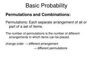
Permutations • Example: • You own three leases (A,B,C) • drill two randomly • without replacement • how many ways can you choose 2 from 3 • (A,B), (A,C), (B,C), (B,A), ( , ), ( , )
Permutations and Combinations • If order matters choose r from n: • Permutations = n!/(n-r)! = 3!/(3-2)! = 3 * 2 * 1/1 • = 6 • If order doesn't matters choose r from n: • Combinations = n!/((n-r)!r!) = 3!/((3-2)!2!) • = 3×2/2 = 3
Multiplication Rule and Independence • Multiplication rule: • P(S1 ∩ S2) = P(S1|S2) * P(S1) • Independence: • P(S1 ∩ S2) = P(S1) * P(S2) • Example: • Are discovering Fe and Cu independent? • P(Fe ∩ Cu) = 1/10 • P(Fe) *P(Cu) = (2/10)*(3/10) = 6/10
Implication of independence • P(Cu|Fe) = P(Cu ∩ Fe) / P(Fe) • = (P(Fe)P(Cu)) / P(Fe) = P(Cu) • marginal probability = conditional
Independent Events • Example: • Russian gas company Gazprom exploring 4 gas fields • one well per field • similar geology – 1/3 chance of success • probability you get a success on the first two wells • success field independent of success in others • P(S1 ∩ S2) = P(S1) *P(S1) = 1/3*1/3 = 1/9
Binomial • Notation: • Probability of success = p • trial = n • without replacement • Formula: • p(X = x) = n!/((n-x)!x!)(p)n(1-p)(n-x)
Binomial • Probability 2 of 4 are successful • (S,S,D,D) = 1/3*1/3*2/3*2/3 • (S,D,S,D) = 1/3*2/3*2/3*1/3 • (D,D,S,S) = 1/3*1/3*2/3*2/3 • (S,D,D,S) = 1/3*2/3*2/3*1/3 • (D,S,S,D) = 1/3*2/3*1/3*2/3 • (D,S,D,S) = 1/3*2/3*1/3*2/3 • P(X = 2) = [4!/((4-2)!2!)](1/3)2(2/3)(n-2) = 0.296
Bayes’ Theorem • Bayes - Making decisions using new sample information. • Example: • Batteries hybrid renewable energy (wind, solar) • Three of your plants build the battery • E1 E2 E3 • Two battery types • regular – r • heavy duty – h
Bayes’ Theorem • Cont. Example: • Factory Types Batteries • r h • E1 200 r 100 h Total 300 • E2 50 r 150 h Total 200 • E3 50 r 50 h Total 100 • h battery comes back on warrantee • Probability battery from plant E2 = P(E2|h)?
Bayes’ Theorem • From definition • P(E2|h) = P(h∩E2) => P(h∩E2) = P(E2|h)P(h) • P(h) • but also P(h∩E2) = P(h|E2)P(E2) • Replace in numerator • P(E2|h) = P(h|E2 )P(E2 ) • P(h)
Bayes’ Theorem • What is P(h) = P(h∩E1) + P(h∩E2 ) + P(h∩E3 ) • But • P(h∩E1) = P(h|E1)P(E1) • P(h∩E2) = P(h|E2)P(E2) • P(h∩E3) = P(h|E3)P(E3)
Bayes’ Theorem • Replace in denominator • P(E2|h) = P(h|E2)P(E2) • P(h|E1)P(E1)+P(h|E2)P(E2)+P(h|E3)P(E3) • = (3/4)(1/3) • (1/2)(1/3) + (1/3)(3/4) + (1/6)(1/2) • = 1/2
Bayes’ Theorem • General formula (h occurs) • P(Ei|h) = P(h|Ei)P(Ei) P(h|E1)P(E1)+P(h|E2)P(E2)+P(h|E3)P(E3) • P(Ei|h) = P(h|Ei)P(Ei) • i(P(h|Ei)P(Ei)
Bayesian Econometrics • Econometrics = wedding model and data • Ei = model, h = data • P(model|data) = P(data|model )P(model) • P(data) • Example: yt = + ei • P(|y) = P(y|)P() • P(y)
Prior and Posterior Distributions • P(|y) = P(y|)P() • P(y) • P(y|) = how well data fits given the model • likelihood function • pick model to maximize • P() = prior beliefs • P(y) no model parameters - treat as exogenous • P(|y) = posterior likelihood*prior