Towards a statistical model of the EGEE load
200 likes | 363 Vues
Towards a statistical model of the EGEE load. C. Germain-Renaud , CNRS & Paris-Sud University E. Vazquez, Supelec David Colling, Imperial College Clermont-Ferrand 11-14 Feb 2008. Overview.

Towards a statistical model of the EGEE load
E N D
Presentation Transcript
Towards a statistical model of the EGEE load C. Germain-Renaud, CNRS & Paris-Sud University E. Vazquez, Supelec David Colling, Imperial College Clermont-Ferrand 11-14 Feb 2008
Overview • General goal: contribute to resource dimensioning, providing differentiated Quality of Service (QoS), middleware-level and user-level scheduling • Through statistical modeling of the EGEE workload. Classical observables are inter-arrival time, service i.e. execution times, load i.e. the job backlog • Intrinsic behavior: users requirement, aggregated • Middleware impact: at the computing elements • A further difficulty: background activity • Through autonomic strategies. Utility-based reinforcement learning is emerging. • gLite provides a unique opportunity for such kind of analysis due to extensive logging (L&B) • The Real Time Monitor developed by GridPP gives easy acces to WMS-integrated traces
The Data • More than 18 million jobs • Timestamps of the major events in the job lifecycle • 1st CE : 626K jobs ce03-lcg.cr.cnaf.infn.it • 2nd CE : 579K jobs lcgce01.gridpp.rl.ac.uk • 4th CE : 384K jobs ce101.cern.ch • 33th CE : 107K jobs ce2.egee.cesga.es CE
Statistics workplan • Descriptive statistics • The EGEE job traffic may share some properties with the Internet traffic: many small jobs,and a significant number of large ones, at all scales • Method: parametric modeling of the nominal behavior as well as the tail behavior of the distributions • Time-dependent structures in the time series • Long-range correlation: Poisson processes, with a possibly non homogeneous or stochastic intensity; and self-similar stochastic models such as fractional Gaussian noises (FGN) and fractional ARIMA processes (ARFIMA).
if else With Distribution tails • Tail: restrict to values larger than u – f(x)= P(X >u + x | X > u) • Large u for load is related to extreme (catastophic) events • Large u for inter-arrival is related to QoS • Theoretical answer: generalized Pareto distribution • x = 0: exponential • x> 0: heavy tailed • If x>1/k, the k-th order moment does not exist
Inter-arrival time Definitely not exponential Probably heavy tailed
Fitting a Pareto distribution u0 = 270s u0 = 1500s The estimation of K should be constant u0 = 1100s u0 = 600s (?)
Pareto fit x = 0.51 x = 0.45 x = 0.55 x = 0.68 (?)
Pareto fit Y quantiles Y quantiles x = 0.51 x = 0.45 X quantiles X quantiles The heavy-tail hypothesis stands Small parameter range Y quantiles Y quantiles x = 0.55 x = 0.68 (?) X quantiles X quantiles
Bursts • Observation : • Inter-arrival times (i.e. times between arrival of two jobs) show evidence of bursty behaviour • Problem : find an appropriate representation of this behaviour • Given a threshold, a burst gathers all those jobs separated one from another by a time shorter than the threshold • For each burst, • Size=number of jobs • Length=duration
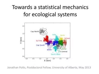
The shape of the average burst size as a function of a threshold does is very similar across the CEs Inter-arrival bursts
Stalactite diagrams • How to read a stalactite diagram: • On a single row, clear areas indicate smaller-sized bursts while darker areas stand for bursts gathering more jobs • Dark vertical areas reveal bursts left undivided by progressive threshold reduction • Interpretation: the more the threshold is reduced, the more jobs are dispatched between shorter bursts EXCEPT for some “stalactites” • Possible use: • Offline detection of exceptional density in inter-arrival times • Model for arrival times • Ongoing work: benchmarking with Cox models • X-Axis : time in days • Y-Axis : threshold in minutes • Color : mean burst size Note : color is normalized on each row
Stalactite diagrams : example Threshold in minutes Time in days
90% percentile Load tails Very contrasted behaviors Ongoing work: classification 20% percentile 60% percentile
Predicting the load • Two naive prediction strategies • Linear from the load history • As the mean of the past executions x number of jobs in the queue • From the load history • We must use only the known load • If t0 is the present date, and t1 the last date where the load was known, t0 - t1 is typically of the order of a few days in active periods • Thus we must extrapolate the load with a horizon of a few days • From the past executions • The correlation of the series of averaged execution times decreases very fast • The horizon for a linear prediction of the execution times is one day at best
On going work: ARCH models • Autoregressive conditional heteroskedasticity (Engle, 1982) Widely used in finance modeling • Fat tails • Time-varying volatility clustering:changes of the same magnitude tend to follow; here the goal is forecasting the variance of the next shock • Leverage effects: volatility negatively correlated with magnitude in change • The one-step-ahead forecast error are zero-mean random disturbances uncorrelated from one period to the next, but not independent
Policy design • Model-based approaches • Predict the performance of the ressources from on-line history and off-line analysis of traces • Model-free approaches • Build a relationship between state of the environment (e.g. grid), available actions, (e.g. jobs to schedule), immediate benefit, and expected long term benefits • Empirical approximation of a value function that gives the expected long-term benefit as a function of the current state • If the dynamics of the system is known, a classical optimization problem • If the dynamic is unknown, reinforcement learning learns the value function by actual actions; a good RL algorithm efficiently samples the (action, value) space
Hard real-time u Soft real-time Best effort fixed t deadline proportional Utility criteria • Time/Utility functions (TUF) – [Jensen, Locke, Tokuda 85] • Utility is a function of the execution delay • Service classes are associated to functions • Other requirements can be included in the utility framework • Weighted fairness is mandatory • Productivity if the scheduling policy is not work-conserving
Experiment • At the CE level - Data: Torque logs LAL 17-26 May 2006 • « Interactive » jobs: execution time less than 15 minutes • Details in CCGRID’08 paper • Further work: evaluate RL at the WMS level