Download
1 / 18
180 likes | 315 Vues
A Statistical Model of Criminal Behavior. M.B. Short, M.R. D’Orsogna, V.B. Pasour, G.E. Tita, P.J. Brantingham, A.L. Bertozzi, L.B. Chayez. Maria Pavlovskaia. Goal. Model the behavior of crime hotspots Focus on house burglaries. Assumptions. Criminals prowl close to home

E N D
A Statistical Model of Criminal Behavior M.B. Short, M.R. D’Orsogna, V.B. Pasour, G.E. Tita, P.J. Brantingham, A.L. Bertozzi, L.B. Chayez Maria Pavlovskaia
Goal • Model the behavior of crime hotspots • Focus on house burglaries
Assumptions • Criminals prowl close to home • Repeat and near-repeat victimization
The Discrete Model • A neighborhood is a 2d lattice • Houses are vertices • Vertices have attractiveness values Ai • Criminals move around the lattice
Criminal Movement A criminal can: • Rob the house he is at - or - • Move to an adjacent house • Criminals regenerate at each node
Criminal Movement • Modeled as a biased random walk
Attractiveness Values • Rate of burglary when a criminal is at that house • Has a static and a dynamic component • Static (A0) - overall attractiveness of the house • Dynamic (B(t)) - based on repeat and near-repeat victimization
Dynamic Component • When a house s is robbed, Bs(t) increases • When a neighboring house s’ is robbed, Bs(t) increases • Bs(t) decays in time if no robberies occur
Dynamic Component • The importance of neighboring effects: • The importance of repeat victimization: • When repeat victimization is most likely to occur: • Number of burglaries between t and t: Es(t)
Computer Simulations Three Behavioral Regimes are Observed: • Spatial Homogeneity • Dynamic Hotspots • Stationary Hotspots
Spatial Homogeneity Dynamic Hotspots Stationary Hotspots
Computer Simulations Three Behavioral Regimes are Observed: • Spatial Homogeneity • Large number of criminals or burglaries • Dynamic Hotspots • Low number of criminals and burglaries • Manifestation of the other two regimes due to finite size effects • Stationary Hotspots • Large number of criminals or burglaries
Continuum Limit In the limit as the time unit and the lattice spacing becomes small: • The dynamic component of attractiveness: • The criminal density:
Continuum Limit • Reaction-diffusion system • Dimensionless version is similar to: • Chemotaxis models in biology (do not contain the time derivative) • Population bioglogy studies of wolfe and coyote territories
Computer Simulations • Dynamic Hotspots are never seen • Spatial Homogeneity or Stationary Hotspots? • Performed linear stability analysis • Found an inequality to distinguish between the cases
Summary • Discrete Model • Computer Simulations • Spatial Homogeneity, Dynamic Hotspots, Stationary Hotspots • Continuum Limit • Dynamic Hotspots are not observed: due to finite size effects • Inequality to distinguish between Homogeneity and Hotspots cases
Applications • House burglaries • Assault with a lethal weapon • Muggings • Terrorist attacks in Iraq • Lootings