Statistical model building
Statistical model building. Marian Scott Dept of Statistics, University of Glasgow Glasgow, Sept 2007. Outline of presentation. Statistical models- what are the principles describing variation empiricism Fitting models- calibration Testing models- validation or verification

Statistical model building
E N D
Presentation Transcript
Statistical model building Marian Scott Dept of Statistics, University of Glasgow Glasgow, Sept 2007
Outline of presentation • Statistical models- what are the principles • describing variation • empiricism • Fitting models- calibration • Testing models- validation or verification • Quantifying and apportioning variation in model and data. • Stochastic and deterministic models. • Model choice
All models are wrong but some are useful(and some are more useful than others) (All data are useful, but some are more varied than others.) a quote from a famous statistician, George Box
Step 1 • why do you want to build a model- what is your objective? • what data are available and how were they collected? • is there a natural response or outcome and other explanatory variables or covariates?
Modelling objectives • explore relationships • make predictions • improve understanding • test hypotheses
Conceptual system Data feedbacks Model inputs & parameters Policy model results
Why model? • Purposes of modelling: • Describe/summarise • Predict - what if…. • Test hypotheses • Manage • What is a good model? • Simple, realistic, efficient, reliable, valid
Value judgements • Different criteria of unequal importance • key comparison often comparison to observational data but • such comparisons must include the model uncertainties and the uncertainties on the observational data (touched on later).
Is the model valid? Are the assumptions reasonable? Does the model make sense based on best scientific knowledge? Is the model credible? Do the model predictions match the observed data? How uncertain are the results? Questions we ask about models
Statistical models • Always includes an term to describe random variation • Empirical • Descriptive and predictive • Model building goal: simplest model which is adequate • used for inference
Physical/process based models • Uses best scientific knowledge • May not explicitly include , or any random variation • Descriptive and predictive • Goal may not be simplest model • Not used for inference
Models Mathematical (deterministic/process based) models tend • to be complex • to ignore important sources of uncertainty Statistical models tend • to be empirical • To ignore much of the biological/physical/chemical knowledge
Stages in modelling • Design and conceptualisation: • Visualisation of structure • Identification of processes (variable selection) • Choice of parameterisation • Fitting and assessment • parameter estimation (calibration) • Goodness of fit
a visual model- atmospheric flux of pollutants • Atmospheric pollutants dispersed over Europe • In the 1970’ considerable environmental damage caused by acid rain • International action • Development of EMEP programme, models and measurements
The mathematical flux model L: Monin-Obukhov length u*: Friction velocity of wind cp: constant (=1.01) : constant (=1246 gm-3) T: air temperature (in Kelvin) k: constant (=0.41) g: gravitational force (=9.81m/s) H: the rate of heat transfer per unit area gasht: Current height that measurements are taken at. d: zero plane displacement
what would a statistician do if confronted with this problem? • ask what the objective of modelling is • look at the data, and data quality • try and understand the measurement processes • think about how the scientific knowledge, conceptual model relates to what we have measured • think about uncertainty
Step 2- understand your data • study your data • learn its properties • tools- graphical
measured atmospheric fluxes for 1997 • measured fluxes for 1997 are still noisy. • Is there a statistical signal and at what timescale?
The Monitoring Networks Sulphur and Nitrogen EMEP: 15 stations in United Kingdom and 4 in Republic of Ireland from 1978 to 1998. (aggregated to monthly means). (SO2, SO4, NO2, NO3, NH4, HNO3+NO3, NH3+NH4) Ozone (O3) UK National Air Quality Information Archive: 8 stations in the United Kingdom corresponding to some of EMEP stations from 1983 to 2007. (hourly data, subsequently aggregated to monthly day and night means).
GB02 Eskdalemuir GB03 Goonhilly GB04 Stoke ferry GB05 Ludlow GB06 Lough Navar GB07 Barcombe Mills GB13 Yarner Wood GB14 High Muffles GB15 Starth Vaich Dam GB16 Glen Dye GB36 Harwell GB37 Ladybower GB38 Lullington Heath GB43 Narberth GB45 Wicken Fen IE01 Valentia Obs. IE02 Turlough Hill IE03 The Burren IE04 Ridge of Capard
THE DATA What evidence is there of a trend in the atmospheric concentrations? • Outliers • Missing values • Discontinuities
Key properties of any measurement • Accuracy refers to the deviation of the measurement from the ‘true’ value • Precision refers to the variation in a series of replicate measurements (obtained under identical conditions)
Accuracy and precision Accurate Inaccurate Precise Imprecise
Evaluation of precision • Analysis of the instrumentation method to make a single measurement, and the propagation of any errors • Repeat measurements (true replicates) – using homogeneous material, repeatedly subsampling, etc…. Precision is linked to Variance (standard deviation)
The nature of measurement • All measurement is subject to uncertainty • Analytical uncertainty reflects that every time a measurement is made (under identical conditions), the result is different. • Sampling uncertainty represents the ‘natural’ variation in the organism within the environment.
The error and uncertainty in a measurement • The error is a single value, which represents the difference between the measured value and the true value • The uncertainty is a range of values, and describes the errors which might have been observed were the measurement repeated under IDENTICAL conditions • Error (and uncertainty) includes a combination of variance and bias
Lack of observations contribute to uncertainties in input data uncertainty in model parameter values Conflicting evidence contributes to uncertainty about model form uncertainty about validity of assumptions Effect of uncertainties
Step 3- build the statistical model • Outcomes or Responses sometimes referred to as ‘dependent variables’. • Causes or Explanationsthese are the conditions or environment within which the outcomes or responses have been observed and are sometimes referred to as ‘independent variables’, but more commonly known as covariates.
Statistical models • In experiments many of the covariates have been determined by the experimenter but some may be aspects that the experimenter has no control over but that are relevant to the outcomes or responses. • In observational studies, these are usually not under the control of the experimenter but are recorded as possible explanations of the outcomes or responses. • we may not know which covariates are important. • recognise that we may build several models before making the final choice
Specifying a statistical models • Models specify the way in which outcomes and causes link together, eg. • Metabolite = Temperature • The = sign does not indicate equality in a mathematical sense and there should be an additional item on the right hand side giving a formula:- • Metabolite = Temperature + Error
Specifying a statistical model • Metabolite = Temperature + Error • In mathematical terms, there will be some unknown parameters to be estimated, and some assumptions will be made about the error distribution • Metabolite = + temperature + • ~ N(0, σ2)- appropriate perhaps? • σ,, are model parameters and are unknown
Model calibration • Statisticians tend to talk about model fitting, calibration means something else to them. • Methods- least squares or maximum likelihood • least squares:- find the parameter estimates that minimise the sum of squares (SS) • SS=(observed y- model fitted y)2 • maximum likelihood- find the parameter estimates that maximise the likelihood of the data
Calibration-using the data • A good idea, if possible to have a training and a test set of data-split the data (e.g. 90%/10%) • Fit the model using the training set, evaluate the model using the test set. • why? • because if we assess how well the model performs on the data that were used to fit it, then we are being over optimistic
How good is my statistical model? • What criteria do we use to judge the value of our model? • may depend on what the model was built to do • Obvious ones • Closeness to the observed data • Goodness of predictions at previously unobserved covariate values • % variation in response explained (R2)
Model validation • what is validation? • Fit the model using the training set, evaluate the model using the test set. • why? • because if we assess how well the model performs on the data that were used to fit it, then we are being over optimistic • assessment of goodness of fit? • residual sums of squares, mean square error for prediction
Model validation splitting the data set, is it possible? • cross-validation • leave–one-out, leave-k-out • split at random, a ‘small’ % kept aside for testing • other methods: bootstrap and jack-knife
an aside- how well should models agree? • 6 physical-deterministic ocean models (process based-transport, sedimentary processes, numerical solution scheme, grid size) used to predict the dispersal of a pollutant • Results to be used to determine a remediation policy for an illegal dumping of “radioactive waste” The what if scenario investigation • The models differ in their detail and also in their spatial scale
Predictions of levels of cobalt-60 • Different models, same input data • Predictions vary by considerable margins • Magnitude of variation a function of spatial distribution of sites
model ensembles • becoming increasingly common in climate, meteorology, to make ‘many’ model runs, different models, different starting conditions and then to ‘average’ the results. • why would we do this?
the statistical approach to model building and selection • in a regression situation, we may have many potential explanatory variables, how do we choose which to include in the final model? • answer may depend on purpose, on how many explanatory variables there may be • identify variables that can be omitted on statistical grounds (no evidence of effect) (see regression sessions with Adrian for testing and CI approaches)- is an effect statistically significant?
the statistical approach to model building and selection • automatic selection procedures can be useful but also potentially dangerous (e.g. stepwise regression, best subset-regression) • they often identify the ‘best’ under a defined criterion in a family of models (like smallest residual sum of squares). • but this ‘best’ model could in an absolute sense be poor.
the statistical approach to model building and selection • other statistical criteria exist for model choice-AIC, DIC, BIC- based on likelihood approaches, can be used to compare non-nested models (ie parameter set of one model is not contained within parameter set of the ‘larger’ model) • need to be careful of ‘dredging’ for significance • remember statistical significance is not always equal to practical importance
Information criterion • In the general case, the AIC is • AIC=2k-2ln(L) • where k is the number of parameters, and L is the likelihood function. • if we assume that the model errors are normally and independently distributed. Let n be the number of observations and RSS be the residual sum of squares. Then AIC becomes • AIC=2k+nln(RSS/n)
AIC • Increasing the number of free parameters to be estimated improves the goodness of fit. Hence AIC not only rewards goodness of fit, but also includes a penalty that is an increasing function of the number of estimated parameters. This penalty discourages overfitting. The preferred model is the one with the lowest AIC value. The AIC methodology attempts to find the model that best explains the data with a minimum of free parameters.
blending the statistical modelling approach to deterministic models • relatively new area (at least for statisticians) • phrased in a Bayesian framework (see later session on Bayesian methods) • makes use of data (very important) and data modelling • still at the research stage (probably most used on climatology)