Comprehensive Guide to Polynomial Models in Regression Analysis
Explore the power of polynomial regression models with a detailed overview of their types, predictors, and interactions. Learn to select the right model using practical examples and validate it effectively.


Comprehensive Guide to Polynomial Models in Regression Analysis
E N D
Presentation Transcript
Model Building Chapter 9 Supplement
Introduction • Regression analysis is one of the most commonly used techniques in statistics. • It is considered powerful for several reasons: • It can cover a variety of mathematical models • linear relationships. • non - linear relationships. • nominal independent variables. • It provides efficient methods for model building
Polynomial Models • There are models where the independent variables (xi) may appear as functions of a smaller number of predictor variables. • Polynomial models are one such example.
Polynomial Models with One Predictor Variable y = b0 + b1x1+ b2x2 +…+ bpxp + e y = b0 + b1x + b2x2 + …+bpxp + e
b2 < 0 b2 > 0 Polynomial Models with One Predictor Variable • First order model (p = 1) • y = b0 + b1x+ e • Second order model (p=2) • y = b0 + b1x + e b2x2+ e
b3 < 0 b3 > 0 Polynomial Models with One Predictor Variable • Third order model (p = 3) • y = b0 + b1x + b2x2+e b3x3 + e
y x1 x2 Polynomial Models with Two Predictor Variables y b1 > 0 • First order modely = b0 + b1x1 + e b2x2 + e b1 < 0 x1 x2 b2 > 0 b2 < 0
First order model, two predictors,and interactiony = b0 + b1x1 + b2x2+b3x1x2 + e x1 Polynomial Models with Two Predictor Variables • First order modely = b0 + b1x1 + b2x2+ e The effect of one predictor variable on y is independent of the effect of the other predictor variable on y. The two variables interact to affect the value of y. X2 = 3 [b0+b2(3)] +[b1+b3(3)]x1 [b0+b2(3)] +b1x1 X2 = 3 X2 = 2 [b0+b2(2)] +b1x1 [b0+b2(2)] +[b1+b3(2)]x1 X2 = 1 X2 = 2 [b0+b2(1)] +b1x1 [b0+b2(1)] +[b1+b3(1)]x1 X2 =1 x1
b5x1x2 + e Second order model with interaction y = b0 + b1x1 + b2x2 +b3x12 + b4x22+ e Polynomial Models with Two Predictor Variables Second order modely = b0 + b1x1 + b2x2 + b3x12 + b4x22 + e X2 = 3 X2 = 3 y = [b0+b2(3)+b4(32)]+ b1x1 + b3x12 + e X2 = 2 X2 = 2 X2 =1 y = [b0+b2(2)+b4(22)]+ b1x1 + b3x12 + e X2 =1 y = [b0+b2(1)+b4(12)]+ b1x1 + b3x12 + e x1
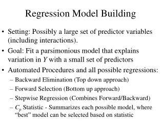
Selecting a Model • Several models have been introduced. • How do we select the right model? • Selecting a model: • Use your knowledge of the problem (variables involved and the nature of the relationship between them) to select a model. • Test the model using statistical techniques.
Selecting a Model; Example • Example: The location of a new restaurant • A fast food restaurant chain tries to identify new locations that are likely to be profitable. • The primary market for such restaurants is middle-income adults and their children (between the age 5 and 12). • Which regression model should be proposed to predict the profitability of new locations?
Revenue Revenue Income age Low Middle High Low Middle High Selecting a Model; Example • Solution • The dependent variable will be Gross Revenue • Quadratic relationships between Revenue and each predictor variable should be observed. Why? • Families with very young or older kids will not visit the restaurant as frequent as families with mid-range ages of kids. • Members of middle-class families are more likely to visit a fast food restaurant than members of poor or wealthy families.
Include interaction term when in doubt,and test its relevance later. Selecting a Model; Example • Solution • The quadratic regression model built is Sales = b0 + b1INCOME + b2AGE + b3INCOME2 +b4AGE2 + b5(INCOME)(AGE) +e SALES = annual gross salesINCOME = median annual household income in the neighborhood AGE= mean age of children in the neighborhood
Selecting a Model; Example To verify the validity of the proposed model for recommending the location of a new fast food restaurant, 25 areas with fast food restaurants were randomly selected. • Each area included one of the firm’s and three competing restaurants. • Data collected included (Xm9-01.xls): • Previous year’s annual gross sales. • Mean annual household income. • Mean age of children
Selecting a Model; Example Xm9-01.xls Collected data Added data
But… Model Validation This is a valid model that can be used to make predictions.
Reducing multicollinearity Model Validation The model can be used to make predictions... …but multicollinearity is a problem!! The t-tests may be distorted, therefore, do not interpret the coefficients or test them. In excel: Tools > Data Analysis > Correlation
Nominal Independent Variables • In many real-life situations one or more independent variables are nominal. • Including nominal variables in a regression analysis model is done via indicator variables. • An indicator variable (I) can assume one out of two values, “zero” or “one”. 1 if a degree earned is in Finance 0 if a degree earned is not in Finance 1 if the temperature was below 50o 0 if the temperature was 50o or more 1 if a first condition out of two is met 0 if a second condition out of two is met 1 if data were collected before 1980 0 if data were collected after 1980 I=
Nominal Independent Variables; Example: Auction Price of Cars A car dealer wants to predict the auction price of a car. Xm9-02a_supp • The dealer believes now that odometer reading and the car color are variables that affect a car’s price. • Three color categories are considered: • White • Silver • Other colors • Note: Color is a nominal variable.
Nominal Independent Variables; Example: Auction Price of Cars • data - revised (Xm9-02b_supp) 1 if the color is white 0 if the color is not white I1 = 1 if the color is silver 0 if the color is not silver I2 = The category “Other colors” is defined by: I1 = 0; I2 = 0
How Many Indicator Variables? • Note: To represent the situation of three possible colors we need only two indicator variables. • Conclusion: To represent a nominal variable with m possible categories, we must create m-1 indicator variables.
Nominal Independent Variables; Example: Auction Car Price • Solution • the proposed model is y = b0 + b1(Odometer) + b2I1 + b3I2 + e • The data White car Other color Silver color
Example: Auction Car Price The Regression Equation From Excel we get the regression equation PRICE = 16701-.0555(Odometer)+90.48(I-1)+295.48(I-2) For one additional mile the auction price decreases by 5.55 cents. A white car sells, on the average, for $90.48 more than a car of the “Other color” category A silver color car sells, on the average, for $295.48 more than a car of the “Other color” category.
Price 16996.48 - .0555(Odometer) 16791.48 - .0555(Odometer) 16701 - .0555(Odometer) Odometer Example: Auction Car Price The Regression Equation From Excel (Xm9-02b_supp) we get the regression equation PRICE = 16701-.0555(Odometer)+90.48(I-1)+295.48(I-2) The equation for a silver color car. Price = 16701 - .0555(Odometer) + 90.48(0) + 295.48(1) The equation for a white color car. Price = 16701 - .0555(Odometer) + 90.48(1) + 295.48(0) Price = 16701 - .0555(Odometer) + 45.2(0) + 148(0) The equation for an “other color” car.
There is insufficient evidence to infer that a white color car and a car of “other color” sell for a different auction price. There is sufficient evidence to infer that a silver color car sells for a larger price than a car of the “other color” category. Example: Auction Car Price The Regression Equation Xm9-02b_supp
Nominal Independent Variables; Example: MBA Program Admission (MBA II) • The Dean wants to evaluate applications for the MBA program by predicting future performance of the applicants. • The following three predictors were suggested: • Undergraduate GPA • GMAT score • Years of work experience • It is now believed that the type of undergraduate degree should be included in the model. Note: The undergraduate degree is nominal data.
Nominal Independent Variables; Example: MBA Program Admission 1 if B.A. 0 otherwise I1 = 1 if B.B.A 0 otherwise I2 = 1 if B.Sc. or B.Eng. 0 otherwise I3 = The category “Other group” is defined by: I1 = 0; I2 = 0; I3 = 0
Nominal Independent Variables; Example: MBA Program Admission MBA-II
Applications in Human Resources Management: Pay-Equity • Pay-equity can be handled in two different forms: • Equal pay for equal work • Equal pay for work of equal value. • Regression analysis is extensively employed in cases of equal pay for equal work.
Human Resources Management: Pay-Equity • Example (Xm9-03_supp) • Is there sex discrimination against female managers in a large firm? • A random sample of 100 managers was selected and data were collected as follows: • Annual salary • Years of education • Years of experience • Gender
Human Resources Management: Pay-Equity • Solution • Construct the following multiple regression model:y = b0 + b1Education + b2Experience + b3Gender + e • Note the nature of the variables: • Education – Interval • Experience – Interval • Gender – Nominal (Gender = 1 if male; =0 otherwise).
Human Resources Management: Pay-Equity • Solution – Continued (Xm9-03) • Analysis and Interpretation • The model fits the data quite well. • The model is very useful. • Experience is a variable strongly related to salary. • There is no evidence of sex discrimination.
Human Resources Management: Pay-Equity • Solution – Continued (Xm9-03) • Analysis and Interpretation • Further studying the data we find: Average experience (years) for women is 12. Average experience (years) for men is 17 • Average salary for female manager is $76,189 Average salary for male manager is $97,832
Stepwise Regression • Multicollinearity may prevent the study of the relationship between dependent and independent variables. • The correlation matrix may fail to detect multicollinearity because variables may relate to one another in various ways. • To reduce multicollinearity we can use stepwise regression. • In stepwise regression variables are added to or deleted from the model one at a time, based on their contribution to the current model.
Model Building • Identify the dependent variable, and clearly define it. • List potential predictors. • Bear in mind the problem of multicollinearity. • Consider the cost of gathering, processing and storing data. • Be selective in your choice (try to use as few variables as possible).
Gather the required observations (have at least six observations for each independent variable). • Identify several possible models. • A scatter diagram of the dependent variables can be helpful in formulating the right model. • If you are uncertain, start with first order and second order models, with and without interaction. • Try other relationships (transformations) if the polynomial models fail to provide a good fit. • Use statistical software to estimate the model.
Determine whether the required conditions are satisfied. If not, attempt to correct the problem. • Select the best model. • Use the statistical output. • Use your judgment!!