III. Model Building
III. Model Building. Model building: writing a model that will provide a good fit to a set of data & that will give good estimates of the mean value of y and good predictions of y for given values of the explanatory variables.


III. Model Building
E N D
Presentation Transcript
Model building: writing a model that will provide a good fit to a set of data & that will give good estimates of the mean value of y and good predictions of y for given values of the explanatory variables.
Why is model building important, both in statistical analysis & in analysis in general? • Theory & empirical research
“A social science theory is a reasoned and precise speculation about the answer to a research question, including a statement about why the proposed answer is correct.” • “Theories usually imply several more specific descriptive or causal hypotheses” (King et al., page 19).
A model is “a simplification of, and approximation to, some aspect of the world.” • “Models are never literally ‘true’ or ‘false,’ although good models abstract only the ‘right’ features of the reality they represent” (King et al., page 49).
Remember: social construction of reality (including alleged causal relations); skepticism; rival hypotheses; & contradictory evidence. • What kinds of evidence (or perspectives) would force me to revise or jettison the model?
Three approaches to model building • Begin with a linear model for its simplicity & as a rough approximation of the y/x relationships. • Begin with a curvilinear model to capture the complexities of the y/x relationships. • Begin with a model that incorporates linearity &/or curvilinearity in y/x relationships according to theory & observation.
The predominate approach used to be to start with a simple model & to test it against progressively more complex models. • This approach suffers, however, from the problem associated with omitted variables in the simpler models. • Increasingly common, then, is the approach of starting with more complex models & testing against simpler models (Greene, Econometric Analysis, pages 151-52).
The point of departure for model-building is trying to grasp how the outcome variable y varies as the levels of an explanatory variable change. • We have to know how to write a mathematical equation to model this relationship.
In what follows, let’s pretend that we’ve already done careful univariate & bivariate exploratory data analysis via graphs & numerical summaries (although, on the other hand, the exercise requires here & there that we didn’t do such careful groundwork…).
Suppose we want to model a person’s performance on an exam, y, as a function of a single explanatory variable, x, the person’s amount of study time. • It may be that the person’s score, y, increases in a straight line as the amount of study time increases from 1 to 6 hours.
If this were the entire range of x values used to fit the equation, a linear model would be appropriate:
What, though, if the range of sample hours increased to 10 hours or more: would a straight-line model continue to be satisfactory? • Quite possibly, the increase in exam score for a unit increase in study time would decrease, causing some amount of curvature in the y/x relationship.
What kind of model would be appropriate? A second-order polynomial, called a quadratic:
: value of y when x’s equal 0; shifts the quadratic parabola up or down the y-intercept : the slop of y on x when x=0 (which we don’t really care about & won’t interpret) : negative, degree of downward parabola; positive, degree of upward parabola
Recall that the model is valid only for the range of x values used to estimate the model. • What does this imply about predictions for values that exceed this range?
Testing a second-order equation If tests significant, do not interpret .. (which represents y’s slope on x1 when x1=0).
Let’s continue with this model-building strategy but change the substantive topic. • We’ll focus on the relationship of average hourly wage to a series of explanatory variables (e.g., education & job tenure with the same employer). • Let’s explore the relationship.
Example: use WAGE1, clear • scatter wage educ || qfit wage educ
. gen educ2=educ^2 . su educ educ2 . reg wage educ educ2 Source SS df MS Number of obs = 526 F( 2, 523) = 65.79 Model 1439.40602 2 719.70301 Prob > F = 0.0000 Residual 5721.00827 523 10.9388303 R-squared = 0.2010 Adj R-squared = 0.1980 Total 7160.41429 525 13.6388844 Root MSE = 3.3074 wage Coef. Std. Err. t P>t [95% Conf. Interval] educ -.6074999 .2414904 -2.52 0.012 -1.08191 -.1330897 educ2 .0490724 .0100718 4.87 0.000 .0292862 .0688587 _cons 5.407688 1.458863 3.71 0.000 2.541737 8.273639
If the second-order term tests significant we don’t we interpret the first-order term. • Why not?
Let’s figure out what the second-order term means in this model. • What do the following graphs say about the relationship of wage to years of education?
Median Band Regression & Lowess Smoothing • Median band regression (scatter mband y x) & lowess smoothing (lowess y x) are two very helpful tools for detecting (1) how a model fits or doesn’t fit to particular segments of the x –values (e.g., poorer to richer persons) & (2) thus non-linearity. • Hence they’re really useful at all stages of exploratory data analysis. • Another option: locpoly y x1
What did the graphs say about the relationship of wage to years of education? • Let’s answer this question more precisely by predicting the direction & magnitude of the wage/education relationship at specific levels of education, identified via ‘su x, detail’ and/or our knowledge of the issue:
. su educ, d . lincom educ*9 + educ2*81 wage Coef. Std. Err. t P>t [95% Conf. Interval] (1) -1.492631 1.388045 -1.08 0.283 -4.219459 1.234197 . lincom educ*12 + educ2*144 wage Coef. Std. Err. t P>t [95% Conf. Interval] (1) -.2235668 1.514447 -0.15 0.883 -3.198713 2.75158 . lincom educ*16 + educ2*256 wage Coef. Std. Err. t P>t [95% Conf. Interval] (1) 2.842547 1.456761 1.95 0.052 -.0192752 5.70437
Don’t get hung up with every segment of the curve. • The curve is only an approximation. Thus it may not fit the data well within any particular range (especially where there are few observations).
Remember, moreover, that Adj R2 was just .198 for this model. • Obviously there are other relevant explanatory variables. Not only do we need to identify them, but we also need to ask: are they independent & linear? independent & curvilinear? or are they interactional?
Interaction Effects • Interaction: the effect of a 1-unit change in one explanatory variable depends on the level of another explanatory variable. • With interaction, both the y-intercept & the regression slope change; i.e. the regression lines are not parallel.
E.g., how do education & job tenure interact with regard to predicted wage? • . gen educXtenure=educ*tenure
. reg wage educ tenure educXtenure Source SS df MS Number of obs = 526 F( 3, 522) = 82.15 Model 2296.41715 3 765.472384 Prob > F = 0.0000 Residual 4863.99714 522 9.31800218 R-squared = 0.3207 Total 7160.41429 525 13.6388844 Adj R-squared = 0.3168 Root MSE = 3.0525 wage Coef. Std. Err. t P>t [95% Conf. Interval] educ .4265947 .0610327 6.99 0.000 .3066948 . 5464946 tenure -.0822392 .0737709 -1.11 0.265 -.2271635 .0626851 educXtenure .0225057 .0059134 3.81 0.000 .0108887 .0341228 _cons -.4612881 .7832198 -0.59 0.556 -1.999938 1.077362
Let’s interpret the model. • If the interaction term tests significant, we don’t interpret its base variables? • Why not? Each base variable represents its y/x slope when the other x=0. We don’t care about this.
To interpret the interaction term, we use ‘su x1, d’ & our knowledge of the subject to identify key levels of educ & tenure (or use one SD above mean, mean, & one SD below mean): • Then we predict the slope-effect of educXtenure on wage at the specified levels, as follows:
How the interaction of mean education with varying levels of tenure relates to average hourly wage: • . lincom educ + (educXtenure*2) • wage Coef. Std. Err. t P>t [95% Conf. Interval] • (1) -.0372278 .062391 -0.60 0.551 -.1597961 .0853406 • . lincom educ + (educXtenure*10) • wage Coef. Std. Err. t P>t [95% Conf. Interval ] • (1) .142818 .0221835 6.44 0.000 .0992382 .1863978 • . lincom educ + (educXtenure*18) • wage Coef. Std. Err. t P>t [95% Conf. Interval] • (1) .3678751 .0503567 7.31 0.000 .2689484 .4668019
How the interaction of mean tenure with varying levels of education relates to average hourly wage: • . lincom tenure + (8*educXtenure) • wage Coef. Std. Err. t P>t [95% Conf. Interval] • (1) .0978065 0303746 3.22 0.001 .0381351 .157478 • . lincom tenure + (12*educXtenure) • wage Coef. Std. Err. t P>t [95% Conf. Interval] • (1) .1878294 .0184755 10.17 0.000 .1515338 .224125 • . lincom tenure + (20*educXtenure) • wage Coef. Std. Err. t P>t [95% Conf. Interval] • (1) .3678751 .0503567 7.31 0.000 .2689484 .4668019
With significant interaction, to repeat, both the regression coefficient & the y-intercept change as the levels of the second interacting variable change. • That is, the regression slopes are unequal. What does this mean in the model for average hourly wage?
Our interaction model yielded an Adj R2 of .317. • Given the non-linearity we’ve uncovered, could we increase the explanatory power by combining quadratic & interaction terms?
. reg wage educ tenure educXtenure educ2 tenure2 Source SS df MS Number of obs = 526 F( 5, 520) = 59.98 Model 2619.24058 5 523.848116 Prob > F = 0.0000 Residual 4541.17371 520 8.73302637 R-squared = 0.3658 Adj R-squared = 0.3597 Total 7160.41429 525 13.6388844 Root MSE = 2.9552 wage Coef. Std. Err. t P>t [95% Conf. Interval] educ -.7069382 .2269283 -3.12 0.002 -1.152747 -.2611293 tenure -.0072781 .0848573 -0.09 0.932 -.1739834 .1594272 educXtenure .0263957 .005787 4.56 0.000 .0150269 .0377645 educ2 .0470478 .0091265 5.16 0.000 .0291184 .0649771 tenure2 -.0050847 .0016688 -3.05 0.002 -.0083632 -.0018062 _cons 5.763382 1.464726 3.93 0.000 2.885874 8.640889
Let’s assess the model’s fit. • Let’s conduct a test of nested models, comparing this new, ‘full’ model to each of the previous, ‘reduced’ models.
Did adding educXtenure, educ2 & tenure2 boost the model’s variance-explaining power by a statistically significant margin? • . test educXtenure educ2 tenure2 • ( 1) educXtenure = 0 • ( 2) educ2 = 0 • ( 3) tenure2 = 0 • F( 3, 520) = 17.47 • Prob > F = 0.0000
Did adding educ2 & tenure2 boost the model’s variance-explaining power by a statistically significant margin over the interaction model? . test educ2 tenure2 ( 1) educ2 = 0 ( 2) tenure2 = 0 F( 2, 520) = 18.48 Prob > F = 0.0000
Valid testing of nested models To conduct a valid test of nested models: • the number of observations for both the complete & reduced models must be equal; • the functional form of y must be the same (e.g., we can’t compare outcome variable ‘wage’ to outcome variable ‘log-wage’).
Comparing non-nested models • How do we compare non-nested models (i.e. models with the same number of explanatory variables), or nested models that don’t meet the criteria for comparative testing? • Use either the AICor BIC test statistics: the smaller the score, the better the model fits. • Download the ‘fitstat’ command (see Long/Freese, Regression Models for Categorical Dependent Variables).