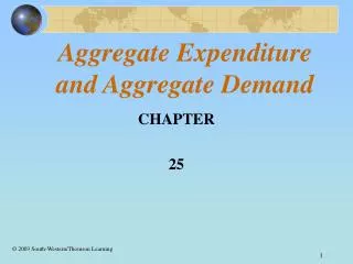
Aggregate Expenditure and Aggregate Demand
Aggregate Expenditure and Aggregate Demand. CHAPTER 25. © 2003 South-Western/Thomson Learning. Aggregate Expenditure and Income. Here we build on the income-consumption connection to uncover the tie between income and total spending Assumptions No capital depreciation No business saving

Aggregate Expenditure and Aggregate Demand
E N D
Presentation Transcript
Aggregate Expenditure and Aggregate Demand CHAPTER 25 © 2003 South-Western/Thomson Learning
Aggregate Expenditure and Income • Here we build on the income-consumption connection to uncover the tie between income and total spending • Assumptions • No capital depreciation • No business saving • Each dollar spent on production translates directly into a dollar of aggregate income GDP equals aggregate income • Investment, government purchases, and net exports are autonomous independent of the level of income
Components of Aggregate Expenditure • To develop the aggregate demand curve, we begin by asking how much aggregate output would be demanded at a given price level • Our objective is to analyze the relationship between aggregate spending in the economy and aggregate income, or real GDP
Aggregate Expenditures • Aggregate expenditures equals the amount that households, firms, governments, and the rest of the world plan to spend on U.S. output at each level of real GDP • Consumption, C • Planned investment, I • Government purchases, G • Net exports, X – M • Consumption is the only spending component that varies with the level of real GDP
Exhibit 1: Table for Real GDP With Net Taxes and Government Purchases (trillions of dollars) • Suppose the price level in the economy is 130 30% higher than in the base year • First column lists a range of possible levels of real GDP symbolized by Y • When we subtract net taxes, column (2), we get disposable income in column (3) • Households only have two possible uses for disposable income • Consumption, MPC assumed to be 4/5 • Saving, MPS assumed to be 1/5
Columns (6), (7), and (8) list the injections into the circular flow: planned investment, government purchases and net exports. Government purchases equals net taxes government’s budget is balanced The final column lists any unplanned inventory adjustment which equals real GDP minus planned aggregate expenditures When the amount people plan to spend equals the amount produced, there are no unplanned inventory adjustments. In our example, this occurs where planned aggregate expenditures and real GDP equal 10.0
Exhibit 1: Table for Real GDP With Net Taxes and Government Purchases (trillions of dollars) • If, however, real GDP is $9.0 trillion • Planned aggregate expenditure is $9.2 trillion firms must reduce inventories to make up the shortfall in output • When the amount produced exceeds planned spending, firms get stuck with unsold goods which become unplanned increases in inventories • For example, if real GDP is $11.0 trillion, planned aggregate expenditure is only $10.8 trillion $0.2 million in output remains unsold firms respond by reducing output and do so until they produce the amount that people want to buy
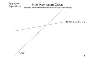
e 10.0 10.0 Exhibit 2: Deriving Aggregate Output This graph is often called the income-expenditure model. The aggregate expenditure line reflects the sum of consumption, investment, government purchases, and net exports C + I + G + (X – M) Planned aggregate expenditure is measured on the vertical axis. Real GDP, measured on the horizontal axis, can be viewed in two ways: 1) the value of aggregate output ,and 2) as the aggregate income generated by that level of output for a given price level Aggregate expenditure (trillions of dollars) 45º 0 Real GDP (trillions of dollars)
e 10.0 10.0 Exhibit 2: Deriving Aggregate Output The special feature of the 45-degree line is that it identifies all points where planned expenditure equals real GDP. C + I + G + (X – M) Aggregate expenditure (trillions of dollars) Aggregate output demanded at any given price level occurs where real GDP equals planned aggregate expenditure, at point e 45º 0 Real GDP (trillions of dollars)
e 10.0 b 9.2 9.0 a 9.0 10.0 Exhibit 2: Deriving Aggregate Output Consider what happens when real GDP is initially less than $10.0 trillion, say $9.0 trillion. Planned aggregate expenditures of $9.2 trillion (point b) exceed real GDP: planned expenditures exceed the amount that firms produce. Because we assume prices will remain constant, firms will reduce inventories. But unplanned inventory reductions cannot continue indefinitely; firms will increase employment increasing income increasing consumer spending. This process will continue until planned spending equals real GDP at point e C + I + G + (X – M) Aggregate expenditure (trillions of dollars) 45º 0 Real GDP (trillions of dollars)
d 11.0 10.8 c e 10.0 10.0 11.0 Exhibit 2: Deriving Aggregate Output When aggregate expenditures exceed real GDP - for example at $11.0 - planned spending (point c on the AE line) falls short of production (point d). Since real GDP exceeds the amount people want to spend, unsold goods accumulate. Rather than allow inventories to pile up indefinitely, firms reduce production, which reduces employment and income. C + I + G + (X – M) Aggregate expenditure (trillions of dollars) 45º 0 Real GDP (trillions of dollars)
Simple Spending Multiplier • If we continue to assume that the price level remains unchanged, we can trace the effects of changes in planned spending on aggregate output demanded • The key point is that like a stone thrown into a still pond, the effect of any shift in planned spending ripples through the economy, generating changes in aggregate output that may far exceed the initial shift in planned spending
a 10.1 0.1 Exhibit 3: Effect of an Increase In Autonomous Investment on Real GDP Demanded Assume that we begin at equilibrium at point e and that firms become more optimistic about future prospects. As a result they increase their planned investment, from I to I'. ) s r a e´ l l o 10.5 d f o C+I´+G+(X-M) s n o i l l i r t ( e r u t i C+I+G+(X-M) d 10.0 e In our example, investment is assumed to have increased by $0.1 trillion per year. What is important to note is that real GDP increased by $0.5 trillion. n e p x e e t a g e r g 45º g A 10.0 0 10.5 Real GDP (trillions of dollars)
e' f c g d a 10.1 b 0.1 10.1 Exhibit 3: Autonomous Increase In Investment Round 1: The upward shift of the AE line means that at the initial real GDP level of $10.0 trillion, planned spending now exceeds output by $0.1 trillion: e a Initially, inventories may be reduced, prompting firms to expand production: a b ) C + I + G + (X – M) s r a l l o 10.5 d f C + I' + G + (X – M) o s n o i l l i r t ( e r u t i d 10.0 e n e e b shows the first round in the multiplier process. Those who receive this additional income spend some of it and save the rest, laying the basis for round two of spending and income. p x e e t a g e r g 45º g A 10.0 0 10.5 Real GDP (trillions of dollars)
e' f c g d a 10.1 b 0.1 10.1 Exhibit 3: Autonomous Increase In Investment Round Two. Given a MPC of 0.8, those who receive the additional income of $100 billion as income will spend a total of $80 billion,shown by the move from point b c. Firms respond by increasing their output by $80 billion: c d. ) C + I + G + (X – M) s r a l l o 10.5 d f C + I' + G + (X – M) o s n o i l l i r t ( e r Round Three and Beyond. This increase of $80 becomes income to resource suppliers. Based on the MPC, we know that four-fifths ($64 billion) will be spent: f g. So long as planned spending exceeds output, production will increase, thereby creating more income, which will generate still more spending u t i d 10.0 e n e p x e e t a g e r g 45º g A 10.0 0 10.5 Real GDP (trillions of dollars)
New Spending Cumulative New Saving Cumulative Round This Round New Spending This Round New Saving 1 100 100 - - 2 80 180 20 20 3 64 244 16 36 10 13.4 446.3 3.35 86.6 0 500 0 100 Exhibit 4: Summary of the Multiplier Effect • Exhibit 4 summarizes the multiplier process, showing the first three rounds, round ten, and the cumulative effect of all rounds • The new spending generated in each round is shown in the second column and the accumulation of new spending appears in the third column • Total new spending after 10 rounds sums to $446.3 billion • But calculating the exact total would require us to work through an infinite series of rounds 8
Simple Spending Multiplier • The cumulative spending resulting from an infinite series of rounds equals 1 / (1 – MPC) which in our example where the MPC was 0.8 1 / 0.2 5 • Thus, the initial increase in planned investment of $100 billion will eventually boost real GDP by 5 times this $100 billion, or $500 billion • Simple Spending Multiplier =1/(1–MPC)
Simple Spending Multiplier • The multiplier depends on the value of the MPC • Specifically, the larger the fraction of an increase in income that is spent each round, the larger the spending multiplier the larger the MPC, the larger the simple multiplier • With an MPC of 0.8, the multiplier is 5 • With an MPC of 0.9, the multiplier is 10 • With an MPC of 0.75, the multiplier is 4
Simple Spending Multiplier • Recall from previous discussions that the MPC and the MPS must add up to 1 • Therefore, we can define the simple spending multiplier in terms of the MPS as follows: • Simple spending multiplier = 1 / MPS
Simple Spending Multiplier • In our example, the multiplier process started because of an increase in investment • The same impact would occur if any one of the components of aggregate expenditures changed • Finally, if the higher level of planned investment is not sustained in future years, real GDP would fall back and the multiplier process would work in reverse
Deriving the Aggregate Demand Curve • Thus far we have used the aggregate expenditure line to determine real GDP demanded for a given price level • What happens to the aggregate expenditure line if the price level changes • As will be seen, for each price level there is a specific aggregate expenditure line which yields a unique real GDP demanded by altering the price level, we can derive the aggregate demand curve
A Higher Price Level • What is the effect of a higher price level on the economy’s aggregate expenditure line and, in turn, on real GDP demanded? • A higher price level • reduces consumption because it reduces the real value of dollar-denominated assets held by households • increases the market rate of interest which reduces investment • makes U.S. goods relatively more expensive abroad imports rise and exports fall
AE (P = 130) e 10.0 e 130 10.0 Exhibit 5: Income-Expenditure and Aggregate Demand Aggregate expenditure (trillions of dollars) In panel (a), the AE function intersects the 45 degree line at point e to yield $10.0 trillion in real GDP demanded. (a) Income-expenditure model 45° 0 Real GDP (trillions of dollars) Panel (b) shows more directly the link between real GDP demanded and the price level. When the price level is 130, real GDP demanded is $10.0 trillion. This combination of price level and real GDP is identified by point e on the aggregate demand curve. 140 Price level (b) Aggregate demand curve Real GDP (trillions of dollars) 0
AE" (P = 120) e" AE (P = 130) AE' (P = 140) e e' 10.5 9.5 10.0 e' e 130 e" 120 AD 9.5 10.0 10.5 If the price level increases to 140? Exhibit 5: Income-Expenditure and Aggregate Demand It reduces consumption, investment, and net exports, as reflected in panel (a) by the downward shift from AE to AE' Aggregate expenditure (trillions of dollars) (a) Income-expenditure model As a result of the decrease in planned spending, real GDP demanded declines from e e' 45° 0 Real GDP (trillions of dollars) If the price level declines to120? 140 It increases consumption, planned investment, and net exports, as reflected panel (a) by the upward shift in the spending line from AE to AE" Price level (b) Aggregate demand curve The increase in planned spending at each income level increases real GDP demanded increases from e e" Real GDP (trillions of dollars) 0
Aggregate Demand and Expenditures • The aggregate expenditure line and the aggregate demand curve portray real output from different perspectives • The aggregate expenditure line shows, for a given price level, how planned spending relates to the level of real GDP in the economy • The aggregate demand curve shows, for various price levels, the quantities of real GDP demanded
Multiplier and Aggregate Demand • Suppose we return to the situation where the price level is assumed to be constant • What we want to do now is trace through the effects of a shift in any of the components of spending on aggregate demand, while assuming that the price level does not change, e.g., we want to look at the multiplier and shifts in aggregate demand
C + I' + G + (X – M) e' 0.1 10.5 AD' 10.5 Exhibit 6: Shifts C + I + G + (X – M) At a price level of 130, the aggregate expenditure line intersects the 45 degree line at point e in panel (a), and yields point e on the aggregate demand curve in panel (b) (a) Income-expenditure model Aggregate expenditure (trillions of dollars) e 45º When one component of aggregate expenditure increases, the AE function shifts upward. Because the price level is assumed constant, the aggregate demand curve shifts from AD to AD' and the new point of equilibrium is shown as e' in both panels. 0 10.0 Real GDP (trillions of dollars) e e´ (b) Aggregate demand curve 130 Price level AD 0 10.0 Real GDP (trillions of dollars)
Limitations of the Multiplier • Our discussion of the simple spending multiplier exaggerates the actual effect we might expect from a given shift in the aggregate expenditure line • We have assumed that the price level remains constant. However, as we will see later, once we incorporate aggregate supply into the analysis, changes in the price level reduce the impact of the multiplier • Leakages such as higher income taxes and increased spending on imports all reduce the size of the multiplier • The spending multiplier takes time to work itself out the process does not occur instantly