Download
1 / 26
260 likes | 279 Vues
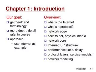
This chapter provides an introduction to systems analysis and control, including mathematical modeling, simulation, and optimization of dynamic systems. Various examples and strategies for systems analysis are discussed.

E N D
Dynamic OptimizationDr. Abebe GeletuIlmenau University of TechnologyDepartment of Simulation and Optimal Processes (SOP) www.tu-ilmenau.de/simulation
Chapter 1: Introduction 1.1 Whatis a system? "A system is a self-contained entity with interconnected elements, process and parts. A system can be the design of nature or a human invention." A system is an aggregation of interactive elements. • A system has a clearly defined boundary. Outside this boundary is the environment surrounding the system. • The interaction of the system with its environment is the most vital aspect. • A system responds, changes its behavior, etc. as a result of influences (impulses) from the environment. www.tu-ilmenau.de/simulation
Course Content • Chapters • Introduction • MathematicalPreliminaries • NumericalMethodsof Differential Equations • Modern MethodsofNonlinearConstrainedOptimization Problems • DirectMethodsfor Dynamic Optimization Problems • Introductionof Model PredictiveControl (Optional) • References: www.tu-ilmenau.de/simulation
1.2. Some examples of systems • Water reservoir and distribution network systems • Thermal energy generation and distribution systems • Solar and/or wind-energy generation and distribution systems • Transportation network systems • Communication network systems • Chemical processing systems • Mechanical systems • Electrical systems • Social Systems • Ecological and environmental system • Biological system • Financial system • Planning and budget management system • etc www.tu-ilmenau.de/simulation
Space and Flight Industries • Dynamic Processes: • Start up • Landing • Trajectory control www.tu-ilmenau.de/simulation
Dynamic Processes: • Start-up • Chemical reactions • Change of Products • Feed variations • Shutdown Chemical Industries www.tu-ilmenau.de/simulation
Industrial Robot • Dynamische Processes: • Positionining • Transportation www.tu-ilmenau.de/simulation
1.3. Why System Analysis and Control? 1.3.1 Purpose of systems analysis: • study how a system behaves under external influences • predict future behavior of a system and make necessary preparations • understand how the components of a system interact among each other • identify important aspects of a system – magnify some while subduing others, etc. www.tu-ilmenau.de/simulation
Strategies for Systems Analysis • System analysisrequiressystemmodelingandsimulationsimulation • A model is a representation or an idealization of a system. • Modeling usually considers some important aspects and processes of a system. • A model for a system can be: • a graphical or pictorial representation • a verbal description • a mathematical formulation • indicating the interaction of components of the system www.tu-ilmenau.de/simulation
1.3.1A. Mathematical Models • The mathematical model of a system • usually leads to a system of equations • describing the nature of the interaction of the system. • These equations are commonly known as governing laws or model equationsof the system. • The model equations can be: • time independent steady-state model equations • time dependent dynamic modelequations • In thiscourse, wearemainlyinterested in dynamicalsystems. Sytemsthatweevolovewith time areknownasdynamicsystems. www.tu-ilmenau.de/simulation
1.3.2. Examples of dynamic models • Linear Differential Equations • Example RLC circuit (Ohm‘sandKirchhoff‘sLaws) www.tu-ilmenau.de/simulation
1.3.2. Examples of dynamic models • Nonlinear Differential equations www.tu-ilmenau.de/simulation
1.3.2. Examples of dynamic models • Nonlinear Differential equations www.tu-ilmenau.de/simulation
1.3.1B Simulation • studies the response of a system under various external influences – input scenarios • for model validation and adjustment – may give hint for parameter estimation • helps identify crucial and influential characterstics (parameters) of a system • helpsinvestigate: instability, chaotic, bifurcationbehaviors • in a systems dynamic as caused by certain external • influences • helps identify parameters that need to becontrolled www.tu-ilmenau.de/simulation
1.3.1B. Simulation ... • In mathematical systems theory, simulation is done • by solving the governing equations of the system for various input scenarios. This requires algorithms corresponding to the type of systems model equation. Numerical methods for the solution of systems of equations and differential equations. www.tu-ilmenau.de/simulation
1.4 Optimization of Dynamic Systems • A system with degrees of freedom can be always manuplated to display certain useful behavior. • Manuplation possibility to control • Control variables are usually systems degrees of freedom. We ask: What is the best control strategy that forces a system display required characterstics, output, follow a trajectory, etc? Methods of Numerical Optimization Optimal Control www.tu-ilmenau.de/simulation
Optimal Control of a space-shuttle 0 1 2 Initial States: The shuttle has a drive engine for both launching and landing. Objective: To land the space vehicle at a given position , say position „0“, where it could be brought halted after landing. Target states: Position , Speed What is the optimal strategy to bring the space-shuttle to the desired state with a minimum energy consumption? www.tu-ilmenau.de/simulation
Optimal Control of a space-shuttle 0 1 2 Model Equations: Then Hence Objectives of the optimal control: • Minimization of the error: • Minimization of energy: www.tu-ilmenau.de/simulation
Problem formulation: Performance function: Model (state ) equations: Initial states: Desired final states: How to solve the above optimal control problem in order to achieve the desired goal? That is, how to determine the optimal trajectories that provide a minimum energy consumption so that the shuttel can be halted at the desired position? www.tu-ilmenau.de/simulation
Optimal Operation of a Batch Reactor www.tu-ilmenau.de/simulation
Optimal Operation of a Batch Reactor • Some basic operations of a batch reactor • feeding Ingredients • adding chemical catalysts • Raising temprature • Reaction startups • Reactor shutdown Chemical ractions: Initial states: Objective: What is the optimal temperature strategy, during the operation of the reactor, in order to maximize the concentration of komponent B in the final product? Allowed limits on the temperature: www.tu-ilmenau.de/simulation
Mathematical Formulation: Objective of the optimization: Model equations: Process constraints: Initial states: Time interval: This is a nonlinear dynamic optimization problem. www.tu-ilmenau.de/simulation
1.5 Optimization of Dynmaic Systems General form of a dynamic optimization problem a DAE system www.tu-ilmenau.de/simulation
1.4. Solution strategies for dynamic optimization problems Solution Strategies IndirectMethods DirectMethods Sequential Method Dynamic Programming Maximum Principle SimultaneousMethod State andcontroldiscretization NonlinearOptimization Solution NonlinearOptimizationAlgorithms www.tu-ilmenau.de/simulation
Solution strategies for dynamic optimization problems • Indirect methods (classical methods) • Calculus of variations ( before the 1950‘s) • Dynamic programming (Bellman, 1953) • The Maximum-Principle (Pontryagin, 1956)1 Lev Pontryagin • Direct (or collocation) Methods (since the 1980‘s) • Discretization of the dynamic system • Transformation of the problem into a nonlinear optimization problem • Solution of the problem using optimization algorithms Verfahren www.tu-ilmenau.de/simulation
1.5. Nonlinear Optimization formulation of dynamic optimization problem • After appropriate renaming of variables we obtain a non-linear programming problem (NLP) Collocation Method www.tu-ilmenau.de/simulation