Empirical Analysis of Market Microstructure: Roll’s and Glosten–Harris Models
130 likes | 311 Vues
Explore empirical market microstructure through Roll’s model and Glosten–Harris model, analyzing bid/ask spreads, order flows, and limit-order book structure. Understand the dynamics of transaction prices and spread in equities and FX markets, along with structural models deviating from the EMH. Discover insights into market impact and empirical findings in equities trading.

Empirical Analysis of Market Microstructure: Roll’s and Glosten–Harris Models
E N D
Presentation Transcript
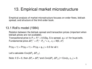
13. Empirical market microstructure Empirical analysis of market microstructure focuses on order flows, bid/ask spread, and structure of the limit-order book. 13.1 Roll’s model (1984) Relation between the bid/ask spread and transaction prices (important when bid/ask prices are not available). Transactional price is Pt = Pt* + 0.5Sqt, S is spread, qt = ±1 for buys/sells. Fundamental price ΔPt* = Pt* - Pt-1* = εt , εt = N(0, σ2) Pr(qt = 1) = Pr(qt =-1) = Pr(qt = qt-1) = 0.5 for all t. Let’s calculate Cov(ΔPt, ΔPt-1). Note: if S = 0, then ΔPt = ΔPt* and Cov(ΔPt, ΔPt-1) = Cov(εt, εt-1) = 0.
13. Empirical market microstructure 13.1 Roll’s model (continued) Possible price paths:
13. Empirical market microstructure 13.1 Roll’s model (continued 2) Joint probability distribution Cov(ΔPt, ΔPt-1)= 0.125( -S2 - S2) = -0.25S2 S = 2
13. Empirical market microstructure 13.1 Roll’s model (continued 3) Roll’s formula => Cov(ΔPt, ΔPt-1) < 0 In equities (Hasbrouck (2007)) and FX (Hashimoto et al (2008)) qt can be correlated (so-called runs), i.e. buys (sells) follow buys (sells): Pr(qt = qt-1) = q ≠ 0.5 Then extension for the Roll’s formula is (de Jong & Rindi (2009)) S = q-1
13. Empirical market microstructure 13.2 Glosten – Harris model (1998) Spread is a dynamic variable that consists of the transitory, Ct, and the adverse selection, Zt, components: St = 2(Ct + Zt). Then Pt = Pt* + (Ct + Zt)qt ; qt = ±1; and Pt* = Pt-1* +Ztqt+ εt In the spirit of the Kyle model, linear dependence on trading size Vt Ct = c0 + c1Vt, Zt = z0 + z1Vt ΔPt = c0 (qt - qt-1) + c1(qtVt - qt-1Vt-1) + z0qt + z1qtVt + εt For a round-trip transaction (qt= 1, qt-1= -1), effective spread is ΔPt= 2Ct + Zt (not St)... Coefficients c0, c1, z0, and z1can be foundfrom empirical data, which show dependence of adverse selection component on trading size.
13. Empirical market microstructure 13.3 Structural models Both Roll’s and Glosten–Harris models depart from the EMH in that the transactional prices are not martingales. In fact, Glosten & Harris offer a price discovery equation. Hasbrouck (1991): information-based price impact can be separated from the inventory-based price impact since the former remains persistent at intermediate time intervals while the latter is transient. The revision of mid-price rt = 0.5[(pta + ptb)/2 – (pt-1a + pt-1b)/2] is described with VAR including the signed order flow xt(positive for buy orders and negative for sell orders) rt= a1rt-1 + a2rt-2 + … + b0xt+ b1xt-1+ … + ε1,t xt= c1rt-1 + c2rt-2 + … + d1xt-1+ d2xt-2+ … + ε2,t Note contemporaneous b0 (but c1).
13. Empirical market microstructure 13.3 Structural models (continued) E(ε1,t) = E(ε2,t) = 0; E(ε1,t ε1,s) = E(ε1,t ε2,s) = E(ε2,t ε2,s) = 0 for t ≠ s If x0= ε2,0 and ε1,t = 0, price impact can be estimated using the cumulative impulse response αm(ε2,t) = An example (Hasbrouck (1999)): Mt = Mt-1 + ε1,t + zε2,t pt = Mt + a(pt - Mt) + bxt xt = -c(pt-1 - Mt-1) + ε2,t (unobservable) efficient price Mt, mid-price pt and trading size xt ε1,t and ε2,t are related to non-trading and trading information 0 < a ≤ 1 (inventory control), b > 0, c > 0
13. Empirical market microstructure 13.3 Structural models (continued 2) If xt> 0, the market maker encourages traders to sell by raising pt. On the other hand, demand is controlled by the negative sign before ‘c’. When a < 1, the model can be expressed as VAR in terms of observable variables: xt = -bcxt-1 - abcxt-2 – a2bcxt-3 +…+ ε2,t rt= (z + b)xt + [zbc – (1 – a)b]xt-1 + a[zbc – (1 – a)b]xt-2 +…+ ε1,t While it has infinite number of terms, higher terms can be neglected as a <1.
13. Empirical market microstructure 13.4 Empirical findings 13.4.1 Equities Intraday US equity trading volumes were U-shaped in the past; currently J- (or even reverse L) shaped. London stock exchange and some Asian markets, too, have reverse-L intraday trading volume patterns (Malinova & Park (2009)). Average trade size: for S&P 500 constituents, it has fallen between 2004 and 2009 from about 1000 shares to below 300 shares. Long-range autocorrelations in signed order flows (Farmer et al (2006), Bouchaud et al (2006)). In equities, order flows => transactional volumes
13. Empirical market microstructure 13.4 Empirical findings 13.4.1 Equities (continued) Market impact is often estimated as a combination of permanent and transitory components with the latter pertinent only to the order that caused it (Kissell & Glantz (2003)). Permanent component may result from the Hasbrouck’s models. Yet... Weber & Rosenow (2005): market impact in equities grows with trading volume as a power law with the exponent lower than one. Bouchaud et al (2004): market impact in equities has power-law decay. Note: market impact is generally estimated as a function of trading volume – i.e. realized market impact. However, the expected market impact (estimated by parsing the order book) is much higher than the realized one (Weber & Rosenow (2005)). This may be explained with that traders attempt to avoid placing their orders at times of low liquidity when the market impactis high.
13. Empirical market microstructure 13.4 Empirical findings 13.4.2 Market impact
13. Empirical market microstructure 13.4 Empirical findings 13.4.3 FX 24x5 market. EUR/USD trading volume has two pronounced maxima, one around 9:00 GMT when trading in London becomes intense and another, even a higher one, at around 15:00 GMT when active trading in London and New York overlap. The USD/JPY trading volume has an additional maximum at around 2:00 GMT, after opening of the Tokyo and Pacific markets. The EUR/USD and USD/JPY spreads are roughly U-shaped and J-shaped, respectively. Autocorrelations in the signed hit flows are practically nonexistent. Autocorrelations in the signed quote flows are much stronger than autocorrelations yet decay much faster than in equity markets. Realized market impact is lower than the expected market impact and has a power-law decay (Schmidt (2010)).