Download
1 / 18
180 likes | 311 Vues
Survival analysis is a statistical method used to estimate the time until events such as death or disease relapse occur. It involves interpreting the hazard function, which represents the instantaneous risk of failure. For patients with conditions like acute myelogenous leukemia (AML), survival data often include censored observations, where the exact event time cannot be determined. Techniques like the Kaplan-Meier estimator allow for effective handling of such data, providing insights into the survival functions of different patient groups. This analysis is critical in clinical research for decision-making.

E N D
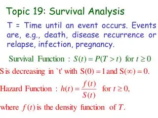
Topic 19: Survival Analysis T = Time until an event occurs. Events are, e.g., death, disease recurrence or relapse, infection, pregnancy.
Interpretation of hazard function Hazard function gives instantaneous risk of failure. For healthy person it is constant whereas for Lukaemia patients, it is decreasing.
In real applications, we don’t expect “used” to be as good as “new”. A more realistic survival variable is Weibull random variable with density
Aim of Survival Analysis is the estimation and comparison of S(t) and h(t). Time until relapse (in weeks) of acute myelogenous leukaemia (AML) patients receiving maintenance chemotherapy 9, 13, 13, 18, 23, 28, 31, 34, 45, 48, 161
(Inherent feature of survival data) Censoring At the end of study, some patients are yet to experience a relapse. Their remission times cannot be ascertained exactly; all we can say is that these times are more than the difference between termination and entry time. We say these remission times are right censored. Note that Censoring can also be the result of dropout and loss to follow up. We need to take into account Censoring while estimating the survival function.
Estimating survival function from censored data (Kaplan-Meier) 9, 13, 13+, 18, 23, 28+, 31, 34, 45+, 48, 161+ Shift the probability mass of the censored observations to the right equally
Kaplan-Meier estimate is also called the product limit estimate Let t(1) < t(2) < t(3), … denote the ordered uncensored time points. Let d(j) denote the number of uncensored events at t(j) and n(j) denote total number of individuals who are at risk at t(j). Then S[t(j)]=[1-d(j)/n(j)]S[t(j-1)]. INTUITION: P[T> u(j)]=[ 1 - P[u(j-1) < T <u(j)|T>u(j-1)] ] P[T>u(j-1)]. Next we compute K-Meier estimator of the AML-data. Order the UNCENSORED times as 9 < 13 < 18 < 23 < 31 < 34 < 48.
Re-distribute to the right algorithm(Kaplan -Meier Estimate) Time
In SPSS, click: Analyze, survival, Kalpan-Meier. In Status, take Var2, where 1 denotes an uncensored event and 0 a censored event. In the `Options’, plot the survival curve.
Next we compare survival Functions of following two groups: Time to relapse (in weeks) Maintained group: 9, 13, 13+, 18, 23, 28+, 31, 34, 45+, 48, 161+ Non-maintained group: 5, 5, 8, 8, 12, 16+, 23, 27, 30, 33, 43, 45
Comparing two groups Maintained group: 9, 13, 13+, 18, 23, 28+, 31, 34, 45+, 48, 161+ Non-maintained group: 5, 5, 8, 8, 12, 16+, 23, 27, 30, 33, 43, 45
SPSS: Click `Status’ for censoring, `Factor’ for two groups and `Options’ for plotting survival curves. Then click `Compare Factor’ for log rank test.