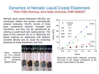
Liquid crystal elastomers
Liquid crystal elastomers. Liquid Crystal elastomer. Normal isotropic elastomer. Monodomain and polydomain samples. Aligned. few microns. Unaligned Polydomain. 1.8. 1.6. 1.4. 1.2. 1.0. 0.8. 0.6. 0.4. 0.2. 0. 2. -1. 0. 1. 10. 10. 10. 10. Mechanical anisotropy.

Liquid crystal elastomers
E N D
Presentation Transcript
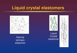
Liquid crystal elastomers Liquid Crystal elastomer Normal isotropic elastomer
Monodomain and polydomain samples Aligned fewmicrons Unaligned Polydomain
1.8 1.6 1.4 1.2 1.0 0.8 0.6 0.4 0.2 0 2 -1 0 1 10 10 10 10 Mechanical anisotropy Anisotropyin monodomain (All samples synthesised by Dr Ali Tajbakhsh) (soft elasticity) D tan d 35º V 50º (like isotropic rubber) 70º 80º Frequency (s-1)
Mechanical anisotropy Master curve constructed using time-Temperature superposition. (Scaled to 35º) 1.8 1.6 1.4 1.2 tan d 1.0 0.8 0.6 0.4 0.2 2 -1 0 1 10 10 10 10 Frequency (s-1)
-1 0 1 2 10 10 10 10 1.8 1.6 1.4 1.2 1 v monodomain 0.8 d monodomain 0.6 0.4 polydomain 0.2 0 Mechanical anisotropy Polydomain compared with monodomain tan d Frequency (s-1)
Stretched Polydomain • Stretching a polydomain material and clamping it during dynamic mechanical analysis – shows same behaviour as monodomain.
35 degrees 1.8 50 degrees 1.6 1.4 1.2 1 0.8 0.6 0.4 0.2 v monodomain d monodomain 0 d stretched polydomain 2 -1 0 1 v stretched polydomain 10 10 10 10 0 polydomain 0 Mechanical anisotropy Stretched Polydomain tan d
Time-resolved experiments:WAXS 2-D intensified CCD detector X-rays Stretch… Oscillatory shear ..and then shear COMPUTER Optical chopper
Azimuthal integration f Fit to: I = a + b * exp(-c * (cos(f-d))^2). “d” shows azimuthal tilt
Variation in tilt angle We can successfully obtain WAXS data at 1s time-resolution without loss of image quality by binning over many cycles. +0.5 mm Strain: movement of arm 0 84 83.5 83 -0.5 mm 82.5 82 81.5 Tilt angle / degrees 81 80s 80.5 10s 40s 80 79.5 79 0 50 100 150 200 250 300 350 Time (degrees of shear cycle)
Phase shift light amplitude Strain 0.35 Sinusoidal strain 0.3 Time-resolved Optical experiments Amplified photodiode Red diode laser Oscillatory stretch COMPUTER Optical chopper
0.4 BUCKLING BUCKLING 0.3 0.2 0.1 Amplitude and phase shift Amplitude / Arbitrary units 0 70º 60º 55º 50º 40º Phase shift (cycles) 0.01 0.1 1 0.01 0.1 1 0 0.01 0.1 1 0.01 0.1 Frequency / s-1 • High temperatures: amplitude independent of frequency; phase shift increases • Medium temperatures: amplitude decreases with frequency; phase shift shows “hump” • Low temperatures: amplitude independent of frequency; phase shift decreases
Model: (assume linear) • Two processes causing changes in transparency on stretching. • One fast (affine deformation? Thinning?) • One slow (disappearance of domain boundaries?) • Both equilibrium transparency linear with strain (for small amplitude)
Transmission of light strain Equilibrium transmission for slow process First-order rate constant amplitude phase shift Derivation of model • (small) sinusoidal imposed strain… • …gives sinusoidal light transmission:
0.4 0.3 0.2 0.1 55º 50º 40º Amplitude data: qualitative fit BUCKLING Amplitude / Arbitrary units 0 f / s-1 0.01 0.1 1 70º 60º 55º 50º 40º • High temperatures: amplitude independent of frequency; • Medium temperatures: amplitude decreases with frequency; • Low temperatures: amplitude independent of frequency; k = 10 k = 1 k = 0.1 k = 0.01 k = 1e-3 1e-4 10
1 / T (K-1) 0.03 0.03 0.03 0.03 ln (k / s-1) 0.02 0.02 0.02 0.02 0.01 0.01 0.01 0.01 Phase shift data: quantitative fit c1 = 2.16 70º k = 6.55 s-1 Data give good fit to model, with temperature-dependent rate constant 60º k = 2.62 s-1 55º k = 0.75 s-1 Phase shift (cycles) = d / 2 p 50º k = 0.26 s-1 0.03 0.02 40º k = 0.022 s-1 0.01 Data consistent with Activation energy EA= 200 kJ mol-1 (assume Arrhenius equation) 0.00 w / s-1 0.01 10 0.1
Phase shift: t-T superposition? Scaled to 50º w / s-1
Fitting our data • Assume t-T superposition, scaled for 50 degrees: + offset At 50º C k = 0.26 s-1 c1 = 17.4 w / s-1
Step-strain Fits first-order mono-exponential I = I0 - A exp(-k t) k increases with temperature 50º C k = 0.17 s-1 40º C k = 0.034 s-1 60º C k = 4.9 s-1 10s 5s 1s 3s 2s 100s 200s
Comparison of first-order rate constants • The sinusoidal and step data agree (within error) • Activation energy 200 kJ mol-1 . (What does this mean?) 1 / T (K-1) ln (k / s-1)