Download
1 / 53
530 likes | 695 Vues
An introduction to Bayesian Networks and the Bayes Net Toolbox for Matlab. Kevin Murphy MIT AI Lab 19 May 2003. Outline. An introduction to Bayesian networks An overview of BNT. Family of Alarm. Burglary. Earthquake. E. B. P(A | E,B). e. b. 0.9. 0.1. e. b. 0.2. 0.8. Radio.

E N D
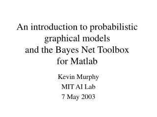
An introduction to Bayesian Networksand the Bayes Net Toolboxfor Matlab Kevin Murphy MIT AI Lab 19 May 2003
Outline • An introduction to Bayesian networks • An overview of BNT
Family of Alarm Burglary Earthquake E B P(A | E,B) e b 0.9 0.1 e b 0.2 0.8 Radio Alarm e b 0.9 0.1 0.01 0.99 e b Call What is a Bayes (belief) net? Compact representation of joint probability distributions via conditional independence Qualitative part: Directed acyclic graph (DAG) • Nodes - random vars. • Edges - direct influence Together: Define a unique distribution in a factored form Quantitative part: Set of conditional probability distributions Figure from N. Friedman
Burglary Earthquake Radio Alarm Call What is a Bayes net? A node is conditionally independent of its ancestors given its parents, e.g. C ? R,B,E | A Hence From 25 – 1 = 31 parameters to 1+1+2+4+2=10
Why are Bayes nets useful? - Graph structure supports - Modular representation of knowledge - Local, distributed algorithms for inference and learning - Intuitive (possibly causal) interpretation • - Factored representation may have exponentially fewer parameters than full joint P(X1,…,Xn) => • lower sample complexity (less data for learning) • lower time complexity (less time for inference)
Burglary Earthquake Radio Alarm Call What can Bayes nets be used for? • Posterior probabilities • Probability of any event given any evidence • Most likely explanation • Scenario that explains evidence • Rational decision making • Maximize expected utility • Value of Information • Effect of intervention • Causal analysis Explaining away effect Radio Call Figure from N. Friedman
MINVOLSET KINKEDTUBE PULMEMBOLUS INTUBATION VENTMACH DISCONNECT PAP SHUNT VENTLUNG VENITUBE PRESS MINOVL FIO2 VENTALV PVSAT ANAPHYLAXIS ARTCO2 EXPCO2 SAO2 TPR INSUFFANESTH HYPOVOLEMIA LVFAILURE CATECHOL LVEDVOLUME STROEVOLUME ERRCAUTER HR ERRBLOWOUTPUT HISTORY CO CVP PCWP HREKG HRSAT HRBP BP A real Bayes net: Alarm Domain: Monitoring Intensive-Care Patients • 37 variables • 509 parameters …instead of 237 Figure from N. Friedman
More real-world BN applications • “Microsoft’s competitive advantage lies in its expertise in Bayesian networks”-- Bill Gates, quoted in LA Times, 1996 • MS Answer Wizards, (printer) troubleshooters • Medical diagnosis • Genetic pedigree analysis • Speech recognition (HMMs) • Gene sequence/expression analysis • Turbocodes (channel coding)
Dealing with time • In many systems, data arrives sequentially • Dynamic Bayes nets (DBNs) can be used to model such time-series (sequence) data • Special cases of DBNs include • State-space models • Hidden Markov models (HMMs)
X1 X2 X3 Y1 Y3 Y2 State-space model (SSM)/Linear Dynamical System (LDS) “True” state Noisy observations
X2 X1 X1 X2 y2 y1 X3 X1 X2 y1 y2 o o X1 X2 Y1 Y3 Y2 o o y1 y2 Example: LDS for 2D tracking Sparse linear Gaussian systems) sparse graphs
X1 X2 X3 Y1 Y3 Y2 Sparse transition matrix ) sparse graph Hidden Markov model (HMM) Phones/ words acoustic signal transitionmatrix Gaussianobservations
Probabilistic graphical models Probabilistic models Graphical models Directed Undirected (Bayesian belief nets) (Markov nets) Alarm network State-space models HMMs Naïve Bayes classifier PCA/ ICA Markov Random Field Boltzmann machine Ising model Max-ent model Log-linear models
Toy example of a Markov net X1 X2 X3 X4 X5 Xi? Xrest| Xnbrs e.g, X1?X4, X5 | X2, X3 Potential functions Partition function
A real Markov net Observed pixels Latent causes • Estimate P(x1, …, xn | y1, …, yn) • Y(xi, yi) = P(observe yi | xi): local evidence • Y(xi, xj) / exp(-J(xi, xj)): compatibility matrixc.f., Ising/Potts model
Burglary Earthquake Radio Alarm Call Inference • Posterior probabilities • Probability of any event given any evidence • Most likely explanation • Scenario that explains evidence • Rational decision making • Maximize expected utility • Value of Information • Effect of intervention • Causal analysis Explaining away effect Radio Call Figure from N. Friedman
X3 X1 X2 Y1 Y3 Y2 Kalman filtering (recursive state estimation in an LDS) • Estimate P(Xt|y1:t) from P(Xt-1|y1:t-1) and yt • Predict: P(Xt|y1:t-1) = sXt-1 P(Xt|Xt-1) P(Xt-1|y1:t-1) • Update: P(Xt|y1:t) / P(yt|Xt) P(Xt|y1:t-1)
Discrete-state analog of Kalman filter O(T S2) time using dynamic programming Forwards algorithm for HMMs Predict: Update:
at|t-1 Xt+1 Xt-1 Xt bt+1 bt Yt-1 Yt+1 Yt Message passing view of forwards algorithm
bt at|t-1 Xt-1 Xt Xt+1 bt Yt-1 Yt+1 Yt Forwards-backwards algorithm Discrete analog of RTS smoother
Distribute Collect root root root root Belief Propagation aka Pearl’s algorithm, sum-product algorithm Generalization of forwards-backwards algo. /RTS smoother from chains to trees - linear time, two-pass algorithm Figure from P. Green
X1 X3 X4 X2 X1 X3 X4 X2 BP: parallel, distributed version Stage 1. Stage 2.
For discrete variables, potentials can be represented as multi-dimensional arrays (vectors for single node potentials) For jointly Gaussian variables, we can usey(X) = (m, S) or y(X) = (S-1m ,S-1) In general, we can use mixtures of Gaussians or non-parametric forms Representing potentials
Manipulating discrete potentials Marginalization Multiplication 80% of time is spent manipulating such multi-dimensional arrays!
Manipulating Gaussian potentials • Closed-form formulae for marginalization and multiplication • O(1)/O(n3) complexity per operation • Mixtures of Gaussian potentials are not closed under marginalization, so need approximations (moment matching)
Semi-rings • By redefining * and +, same code implements Kalman filter and forwards algorithm • By replacing + with max, can convert from forwards (sum-product) to Viterbi algorithm (max-product) • BP works on any commutative semi-ring!
Inference in general graphs • BP is only guaranteed to be correct for trees • A general graph should be converted to a junction tree, by clustering nodes • Computationally complexity is exponential in size of the resulting clusters (NP-hard)
Approximate inference • Why? • to avoid exponential complexity of exact inference in discrete loopy graphs • Because cannot compute messages in closed form (even for trees) in the non-linear/non-Gaussian case • How? • Deterministic approximations: loopy BP, mean field, structured variational, etc • Stochastic approximations: MCMC (Gibbs sampling), likelihood weighting, particle filtering, etc - Algorithms make different speed/accuracy tradeoffs - Should provide the user with a choice of algorithms
Learning • Parameter estimation • Model selection (structure learning)
Parameter learning iid data Conditional Probability Tables (CPTs) If some values are missing(latent variables), we must usegradient descent or EM to compute the (locally) maximum likelihood estimates Figure from M. Jordan
Structure learning (data mining) Genetic pathway Gene expression data Figure from N. Friedman
Structure learning • Learning the optimal structure is NP-hard (except for trees) • Hence use heuristic search through space of DAGs or PDAGs or node orderings • Search algorithms: hill climbing, simulated annealing, GAs • Scoring function is often marginal likelihood, or an • approximation like BIC/MDL or AIC Structural complexity penalty
Summary:why are graphical models useful? - Factored representation may have exponentially fewer parameters than full joint P(X1,…,Xn) => • lower time complexity (less time for inference) • lower sample complexity (less data for learning) - Graph structure supports • Modular representation of knowledge • Local, distributed algorithms for inference and learning • Intuitive (possibly causal) interpretation
The Bayes Net Toolbox for Matlab • What is BNT? • Why yet another BN toolbox? • Why Matlab? • An overview of BNT’s design • How to use BNT • Other GM projects
What is BNT? • BNT is an open-source collection of matlab functions for inference and learning of (directed) graphical models • Started in Summer 1997 (DEC CRL), development continued while at UCB • Over 100,000 hits and about 30,000 downloads since May 2000 • About 43,000 lines of code (of which 8,000 are comments)
Why yet another BN toolbox? • In 1997, there were very few BN programs, and all failed to satisfy the following desiderata: • Must support real-valued (vector) data • Must support learning (params and struct) • Must support time series • Must support exact and approximate inference • Must separate API from UI • Must support MRFs as well as BNs • Must be possible to add new models and algorithms • Preferably free • Preferably open-source • Preferably easy to read/ modify • Preferably fast BNT meets all these criteria except for the last
A comparison of GM software www.ai.mit.edu/~murphyk/Software/Bayes/bnsoft.html
Summary of existing GM software • ~8 commercial products (Analytica, BayesiaLab, Bayesware, Business Navigator, Ergo, Hugin, MIM, Netica), focused on data mining and decision support; most have free “student” versions • ~30 academic programs, of which ~20 have source code (mostly Java, some C++/ Lisp) • Most focus on exact inference in discrete, static, directed graphs (notable exceptions: BUGS and VIBES) • Many have nice GUIs and database support BNT contains more features than most of these packages combined!
Why Matlab? • Pros • Excellent interactive development environment • Excellent numerical algorithms (e.g., SVD) • Excellent data visualization • Many other toolboxes, e.g., netlab • Code is high-level and easy to read (e.g., Kalman filter in 5 lines of code) • Matlab is the lingua franca of engineers and NIPS • Cons: • Slow • Commercial license is expensive • Poor support for complex data structures • Other languages I would consider in hindsight: • Lush, R, Ocaml, Numpy, Lisp, Java
BNT’s class structure • Models – bnet, mnet, DBN, factor graph, influence (decision) diagram • CPDs – Gaussian, tabular, softmax, etc • Potentials – discrete, Gaussian, mixed • Inference engines • Exact - junction tree, variable elimination • Approximate - (loopy) belief propagation, sampling • Learning engines • Parameters – EM, (conjugate gradient) • Structure - MCMC over graphs, K2
X Q Y Example: mixture of experts softmax/logistic function
X Q Y 1. Making the graph X = 1; Q = 2; Y = 3; dag = zeros(3,3); dag(X, [Q Y]) = 1; dag(Q, Y) = 1; • Graphs are (sparse) adjacency matrices • GUI would be useful for creating complex graphs • Repetitive graph structure (e.g., chains, grids) is bestcreated using a script (as above)
X Q Y 2. Making the model node_sizes = [1 2 1]; dnodes = [2]; bnet = mk_bnet(dag, node_sizes, … ‘discrete’, dnodes); • X is always observed input, hence only one effective value • Q is a hidden binary node • Y is a hidden scalar node • bnet is a struct, but should be an object • mk_bnet has many optional arguments, passed as string/value pairs
X Q Y 3. Specifying the parameters bnet.CPD{X} = root_CPD(bnet, X); bnet.CPD{Q} = softmax_CPD(bnet, Q); bnet.CPD{Y} = gaussian_CPD(bnet, Y); • CPDs are objects which support various methods such as • Convert_from_CPD_to_potential • Maximize_params_given_expected_suff_stats • Each CPD is created with random parameters • Each CPD constructor has many optional arguments
X 4. Training the model load data –ascii; ncases = size(data, 1); cases = cell(3, ncases); observed = [X Y]; cases(observed, :) = num2cell(data’); Q Y • Training data is stored in cell arrays (slow!), to allow forvariable-sized nodes and missing values • cases{i,t} = value of node i in case t engine = jtree_inf_engine(bnet, observed); • Any inference engine could be used for this trivial model bnet2 = learn_params_em(engine, cases); • We use EM since the Q nodes are hidden during training • learn_params_em is a function, but should be an object
X Q Y 5. Inference/ prediction engine = jtree_inf_engine(bnet2); evidence = cell(1,3); evidence{X} = 0.68; % Q and Y are hidden engine = enter_evidence(engine, evidence); m = marginal_nodes(engine, Y); m.mu % E[Y|X] m.Sigma % Cov[Y|X]
Other kinds of models that BNT supports • Classification/ regression: linear regression, logistic regression, cluster weighted regression, hierarchical mixtures of experts, naïve Bayes • Dimensionality reduction: probabilistic PCA, factor analysis, probabilistic ICA • Density estimation: mixtures of Gaussians • State-space models: LDS, switching LDS, tree-structured AR models • HMM variants: input-output HMM, factorial HMM, coupled HMM, DBNs • Probabilistic expert systems: QMR, Alarm, etc. • Limited-memory influence diagrams (LIMID) • Undirected graphical models (MRFs)
Summary of BNT • Provides many different kinds of models/ CPDs – lego brick philosophy • Provides many inference algorithms, with different speed/ accuracy/ generality tradeoffs (to be chosen by user) • Provides several learning algorithms (parameters and structure) • Source code is easy to read and extend