Fluid Mixing
Fluid Mixing. Greg Voth Wesleyan University. Voth et al. Phys Rev Lett 88:254501 (2002). Chen & Kraichnan Phys. Fluids 10:2867 (1998). Why study fluid mixing?. Nigel listed three fundamental processes that engineers need to optimize that depend on turbulence: Turbulent Combustion


Fluid Mixing
E N D
Presentation Transcript
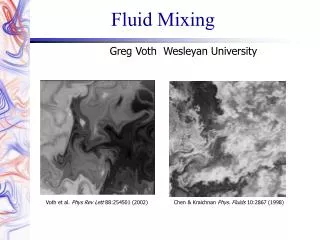
Fluid Mixing Greg Voth Wesleyan University Voth et al. Phys Rev Lett 88:254501 (2002) Chen & Kraichnan Phys. Fluids 10:2867 (1998)
Why study fluid mixing? Nigel listed three fundamental processes that engineers need to optimize that depend on turbulence: • Turbulent Combustion • Environmental Transport • Drag on transportation vehicles • I would argue that each of these is primarily a problem of transport and mixing: • Turbulent Combustion is a transport and mixing of fuel, oxidizer, and thermal energy • Environmental Transport is obviously a mixing problem. • Drag on transportation vehicles is even the turbulent transport of momentum.
Equations for Passive Scalar Transport Advection Diffusion: Navier-Stokes : Incompressibility:
Equations for Passive Scalar Transport Advection Diffusion: Navier-Stokes : Incompressibility: New Dimensionless Parameter: Peclet Number
Equations for Passive Scalar Transport Advection Diffusion: Navier-Stokes : Incompressibility: For small diffusivity, the advection diffusion equation reduces to conservation of the scalar along Lagrangian trajectories.
Scalar Dissipative Anomaly In turbulence, the energy dissipation rate is independent of the viscosity (when the viscosity is reasonably small) even though the viscosity enters the definition of the energy dissipation rate: Similarly, the scalar dissipation rate is independent of the diffusivity (when the diffusivity is reasonably small) even though the viscosity enters its definition: Doniz, Sreenivasan and Yeung JFM 532:199 (2005)
Kolmogorov-Obukhov-Corrsin scaling for passive scalar statistics Scalar Spectrum in the inertial range: (For high Re and Pe) Scalar Structure Functions in the inertial range: Actually: Intermittency of thepassive scalar field is stronger than that of thevelocity field. Warhaft Annu. Rev. Fluid Mech. 32:203 (2000)
Scalar Anisotropy Measurements in a wind tunnel with a mean scalar gradient up to Rl = 460 show the odd moments of the scalar derivative do not go to zero at small scales, indicating persistent anisotropy. Need still higher Re? Intermittency effects?Active Grid Turbulence? In any case, scalar fields generally require higher Reynolds numbers to see isotropy or Kolmogorov scaling. Warhaft. Annu. Rev. Fluid Mech. 32:203–240 (2000)
Lagrangian Descriptions • Fluid mixing is fundamentally a Lagrangian phenomenon…but traditional analysis of turbulent mixing has analyzed the instantaneous spatial structure of the scalar field. Why? • Primarily, Lagrangian data has simply been unavailable • This has changed in the last 25 years…with the availability of numerical simulations and experimental tools for particle tracking. • But the theory was developed before any reliable data was available…why was the Lagrangian description of mixing ignored? • Kolmogorov’s second mistake…see readings for Thursday
Outline of my talks this week Rest of this talk: Lagrangian desciptions of chaotic mixing Patterns in fluid mixing Stretching fields and the Cauchy strain tensors What controls mixing rates Thursday morning and afternoon: Lagrangian descriptions of turbulent flows Lagrangian Kolmogorov Theory Tools for measuring particle trajectories Motion of non-tracer particles in turbulence
Lagrangian descriptions of chaotic mixing Dense, conducting lower layer (glycerol, water, and salt, 3 mm thick) Less dense, non-conducting upper layer (glycerol and water, 1 mm thick) Electrodes Magnet Array Top View: Periodic forcing: Brandeis University, 2002
Persistent Patterns Evolution of dye concentration field Same data updated once per period.
Observations • Dye pattern develops filaments which are stretched and folded until they are small enough that diffusion removes them. • A persistent pattern develops in which transport and stretching balances diffusion. • The overall contrast decays, while the spatial pattern remains unchanged. • Image can be decomposed into a function of space times a function of time. Questions: What determines the geometry of the persistent pattern? What controls the decay rate?
Raw Particle Tracking Data • ~ 800 fluorescent particles tracked simultaneously. • Positions are found with 40mm accuracy. • ~15,000 images: 40-80 images per period of forcing, and 240 periods. • Phase Averaging: 800*240 = 105 particles tracked at each phase. • The flow is time periodic and so exactly the same flow can be used in both dye imaging and particle tracking measurements.
Velocity Fields: Phase averaging allows us to obtain highly accurate time-resolved velocity fields 0.9 cm/sec 0 cm/sec (p=5, Re=56)
Particle Displacement Map • Lines connect position of each measured particle with its position one period later: Poincaré Map. • Color codes for distance traveled in a period: • Blue Small Distance Red Large Distance
Structures in the Poincaré Map Hyperbolic Fixed Points Elliptic Fixed Points
Manifolds of Hyperbolic Fixed Points Unstable Manifold Stable Manifold
Hamiltonian Chaos • Henri Poincaré first identified the hyperbolic fixed points and their manifolds as central to understanding chaos in Hamiltonian systems in a memoir published in 1890. • His interest was in planetary motion and the three body problem, but structures like these are seen in many other problems: • Charged particles in magnetic fields • Quantum systems • But why do these different systems exhibit the same organizing structures? Henri Poincaré (1854-1912) (from Barrow-Green, Poincaré and the three body problem, AMS 1997)
Why do these systems show similar structures? Fluid Mixing Hamiltonian System Real Space Phase Space GeneralizedMomentum, p y x Generalized Position, q Stream Function Equations: Hamilton’s Equations: (Aref, J. Fluid Mech, 1984)
Manifold Structure and Chaos Regular (Non-chaotic) Chaotic
Can we extract manifolds in experiments? • These manifolds have been hard to extract from experiments. They are fundamentally Lagrangian structures. • We could simply search for fixed points and construct the manifolds of each fixed point, but there is a more elegant way: The manifolds consist of fluid elements that experience large stretching (Haller, Chaos 2000) • ... So, we want to measure the stretching fields experienced by fluid elements
Calculating Stretching L0 L Stretching = lim (L/L0) L0 0
Practice with the Cauchy Strain Tensor • What is the Right Cauchy Green Strain Tensor for a uniform strain field:
Practice with the Cauchy Strain Tensor • What is the Right Cauchy Green Strain Tensor for a uniform strain field:
Finite Time Lyapunov Exponent • What is the Right Cauchy Green Strain Tensor for a uniform strain field:
Stretching Field • Stretching is organized in sharp lines. • Stretching Field labels the unstable manifold. • Structure in the stretching field are sometimes called Lagrangian Coherent Structures Re=45, p=1, Dt=3
Unstable manifold and the dye concentration field Brandeis University, 2002
Animation of manifold and dye field • Lines of large past stretching (unstable manifold) are aligned with the contours of the concentration field. • This is true at every time (phase). Brandeis University, 2002
Fixed points and stretching Fixed points dominate the stretching field because particles remain near them for a long time and so are stretched in a single direction. So points near the unstable manifold have large past stretching, and points near the stable manifold have large future stretching. Brandeis University, 2002
Definition of Stretching Stretching = lim (L/L0) L L0 0 Past Stretching Field: Stretching that a fluid element has experienced during the last Dt. Future Stretching Field: Stretching that a fluid element will experience in the next Dt. L0
Future and Past Stretching Fields • Future Stretching Field (Blue) marks the stable manifold • Past Stretching Field (Red) marks the unstable manifold • This pattern is appropriately named a “heteroclinic tangle”.
At Larger Reynolds Number • Stretching fields continue to form sharp lines that mark the manifolds of the flow. • Contours of dye concentration field continue to be aligned by the stretching field. Re=100, p=5
Application to 2D Turbulent Flows Quasi-2D turbulence in a rotating tank Mathur et al, PRL 98:144502 (2007)
Monterey Bay Lekien Couliette and Shadden NY Times September 28, 2009
Summary so far: What determines the geometry of the scalar patterns observed in fluid mixing? • The orientation of the striations in the patterns aligns with lines of large Lagrangian stretching. • In 2D time periodic flows the lines of large stretching match the manifolds that have been the focus of a large amount of work in dynamical systems and chaos. • The Lagrangian stretching can be extracted experimentally with careful optical particle tracking. But what controls the decay rate?
Decay of the Dye Concentration Field (p=5) The functional form can be adequately parameterized by an exponential plus constant.
Predicting Mixing Rates • There is a theory that has been successful in predicting mixing rates in simulated flows: Antonsen et al. (Phys. Fluids8, 3094, 1996) • Takes as input the distribution of Finite Time Lyapunov Exponents of the flow, P(h,t). • Calculates the rate at which scalar variance is transferred to smaller scales by stretching: • Since we have measured the Lyapunov exponents in our flow, we can directly calculate the predicted mixing rate …But it is larger than the observed mixing rate by a factor of 10. Why? • The problem is that transport down scale by stretching is not the rate limiting step in our flow.
Evolution of the Horizontal Concentration Profile Dye pattern approaches a sinusoidal horizontal profile… which is the solution of the diffusion equation in a closed domain . A simple effective diffusion process might be a better model for the mixing rate. t=0, dotted line t = 6 periods, solid line t=36 periods, bold line
Measuring the Effective Diffusivity Then use to find the decay rate of the slowest decaying mode: p=5, Re=100 p=2, Re=100
Comparison of experiment with predictions from effective diffusivity So the mixing rate is determined by effective diffusion, which is a measure of system scale transport, not by stretching which controls the small scale structure of the scalar field. There is an important lesson here: Physicists like the small scales of turbulence. They sometimes shows elegant universality. But often, the quantities that matter are controlled by the large scales.
Source of the Persistent Patterns • The persistent patterns in this system were observed to be • But two very different processes are both contributing to : • Small Scale: Stretching leads to alignment of the contours of concentration with the unstable manifold. • Large Scale: Effective diffusion leads to a sinusoidal pattern with one half wavelength across the system. • Both processes individually create persistent patterns. The large scale pattern decays with time. Rothstein et al, Nature, 401:770 (1999)
Surprises in the Mixing Rates No dramatic change in mixing rate when flow bifurcates to period 2. (p=5, Re=115)
Surprises in the Mixing Rates Or when it becomes turbulent (loses time periodicity). (p=5, Re=170)