Download
1 / 20
240 likes | 420 Vues
Two-dimensional Model for Liquid-Rocket Transverse Combustion Instability by W. A. Sirignano and P. Popov Mechanical and Aerospace Engineering University of California, Irvine Supported by Air Force Office of Scientific Research Dr. Mitat Birkan , Program Manager.

E N D
Two-dimensional Model for Liquid-Rocket Transverse Combustion Instabilityby W. A. Sirignano and P. PopovMechanical and Aerospace EngineeringUniversity of California, IrvineSupported by Air Force Office of Scientific Research Dr. MitatBirkan, Program Manager
Goals of Current UCI Combustion Instability Research • Develop “simplified” liquid-rocket numerical models of combustion dynamics to test stochastic approaches and demonstrate the triggering of combustion instabilities. • Examine nonlinear stability with initial conditions matching linear modes. Identify parameter domains allowing triggering. • Examine nonlinear stability with initial conditions of local Gaussian-shaped disturbance. Identify parameter domains allowing triggering. • Future: Extend the model with the inclusion of stochastic terms representing combustion noise and large-amplitude random perturbations. • Future: Investigate the statistical data for markers of complex system behavior, e.g. power laws. • Future: Extend the work to more detailed combustion dynamics models in collaboration with Georgia Tech and HyPerComp.
Nonlinear Combustion Instability and Triggering Action Princeton experiment, circa 1961. A “bomb” (gunpowder contained with burst disk) is used as the trigger. Instability initiates in various ways, depending upon the operational parameter domain: (1) oscillations that grow from normal combustion noise are named linear or spontaneous instabilities; (2) oscillations initiated only by disturbances larger than noise are named nonlinear or triggered instabilities. All limit-cycle oscillations are nonlinear; “linear” and “nonlinear” refer to initiation.
EARLY THEORIESNonlinear limit cycles were first predicted by Crocco & students inthe 1960s using perturbation methods: Sirignano, Zinn, and Mitchell dissertations. Triggering and stable and unstable limit cycles were predicted.Later, Zinn & Powell followed by Culick and co-workers used a Galerkin method to predict transient behavior as well.Except for one portion of Sirignano’s work, all the models used heuristic representations of combustion: e.g., n, τ model.
Model Equation System • The model equations retain essential physics for the combustion dynamics but eliminate much of the secondary physics which could be added in later studies. This model should allow the testing of our statistical approaches before we engage in a full analysis. • The focus is on transverse oscillations in a cylindrical chamber allowing averaging over the axial direction and reduction to an unsteady, two-dimensional problem in the transverse polar coordinates. • Kinematic waves are neglected leaving only the longer acoustic waves. These kinematic waves travel primarily in the axial direction and because of larger gradients (i.e., shorter wavelengths) are more likely to be vitiated by turbulent mixing. • Viscosity, heat-conductive, and turbulent-mixing effects on the longer acoustic waves are neglected. • A model for co-axial stream turbulent mixing and reaction is developed and employed for a multi-injector configuration. • A simplified “short” multi-orifice nozzle boundary condition is used.
Nonlinear Wave Equation for Pressure E is the energy per unit volume per unit time released by the combustion process. Modelling of E is required. Momentum equations for radial and azimuthal velocities Triggering disturbance could appear in several ways: -- Introduction through reacting, mixing flow-field condition -- Introduction through injector-face boundary condition. -- An intermittent blockage in nozzle flow.
We test wave dynamics with P = (p-p0)/p0 and using a polynomial function E(p) = a P4 – bP3 + cP2 + dPTriggering can occur; stable and unstable limit cycles and transients are captured.
Co-axial Mixing ModelEnergy and Species Equations Uniform pressure over jet One-step reaction Le = 1 Use eddy diffusivity for D Ambient gas oscillates isentropically. P and T are collapsed to one function of entropy.
Schvab-Zel’dovich Variables S-Z formulation plus Oseen approximation reduces three nonlinear PDEs to one nonlinear PDE and two linear, homogeneous PDEs. We may use Green’s function for two equations or numerical integration for all three equations.
Sinusoidal pressure of frequency f . • Two characteristic combustion times appear:τMfor turbulent mixing, τRfor chemical reaction. • A time-lag results: the energy release • rate E lags the pressure p oscillation. • Reaction rate pre-exponental factor is varied from experimental value to explore frequency response for two • time ratios: fτM andfτR . • E maximizes in a certain parameter domain for the two time ratios. • The black line shows the path as frequency varies for the given co-axial • injector design, chamber conditions, • and propellants. Frequency Response of Single Injector
CONFIGURATION: Ten oxygen-methane co-axial injectors • are placed in a combustion • chamber. The model equation is • solved with a co-axial mixing and • reaction for the heat-release. • Chamber length is 0.5m • and diameter is 0.28m . • Injector outer diameter, 1.1cm • Injector inner wall 0.898 cm • Inner flow of gaseous oxygen, • Outer flow of methane gas • “Short” multi-orifice nozzle • Steady-state pressure is • 200atm, temperature is 2000K • First, an individual injector is examined subject to a prescribed • pressure oscillation; then, the analysis is made with ten injectors • coupled to the chamber wave dynamics.
An initial condition of a 1T mode with sufficient amplitude results in triggering. Below a threshold for initial amplitude, decay and stability result. Above the threshold, a stable limit cycle develops. The frequency spectrum analysis shows that nonlinear resonance, in this case, produces a 1T mode, a 2T mode , and a sub-harmonic with frequency equal to difference of 1T and 2T frequencies. Ten-injector Simulation
Sub-harmonics and Nearly Periodic Limit Cycles -- A sub-harmonic mode often appears in nonlinear resonance with a frequency equal to the sum or difference of integer multiples of natural frequencies. -- The presence of the 1T, 2T, and sub-harmonic modes prevents a periodic behavior.. If one natural mode dominates, a nearly periodic behavior results. -- Linear theory does not predict the existence of harmonics for circular cylinders or sub-harmonics for any chamber. -- Galerkin methods require the assumption of the modes present; they do not predict the presence independently. Left: disturbance decays Right: growth occurs with new modes and aperiodic behavior
Pure Second Tangential (2T) Mode is the Initial ConditionTriggering is possible.Nonlinear resonance induces fourth tangential mode plussecond harmonic of 2T.No 1T or sub-harmonic.
Comparison of Variations in E and p -- E is found to lag p in time t and position θ for tangential spinning modes. Example with 2T mode below. -- Energy release is localized in the ten injector streams but differences from one stream to another occur due to pressure phasing.
Test with Variation in Reaction Time-- 1T mode is initial condition.-- Chemical kinetic constant is changed causing longer reaction time.-- The black line in contour plot adjusts and 2T position moves to less sensitive region.-- Consequently, nonlinear resonance does not include 2T and sub-harmonic.-- Nonlinear resonance now involves energy transfer to harmonics of 1T mode.
Local Abrupt Disturbance Local Gaussian-shaped disturbance is provided initially. A direction of initial motion ϴ and an initial amplitude are chosen. For ϴ < 10o , stability occurs. For 10o < ϴ< 43o, 1T mode triggering occurs. For ϴ> 43o, 1T mode plus 1st Radial mode triggering occur with a resulting larger limit-cycle amplitude.
Conclusions from model-equation solution with co-axial injection, mixing and reaction • A nonlinear acoustics model for transverse modes and a co-axial model for propellant mixing and reaction are used to study combustion dynamics with a ten-injector geometry. • Triggering of first tangential mode (1T) and the second tangential mode (2T) is possible; both stable and unstable limit cycles are identified. The stable limit behavior is not always exactly periodic. • Two characteristic combustion times are found and prove to be critical. Accordingly, a time-lag in the combustion response is found. • Depending on characteristic time and frequency values, nonlinear resonance can transfer energy to second tangential mode (2T) and to a sub-harmonic mode. Or energy can be transferred to higher harmonics. The instability occurs for a frequency where the heat-release response to pressure variation is very strong. • Triggering can result from either disturbances with well defined profiles corresponding to natural modes or localized disturbances. • Directional travel orientation of a local disturbance is consequential for triggering. Different stability and different limit cycles can be induced.
CURRENT WORK DIRECTIONS UCI is developing the stochastic framework with the Polynomial Chaos Expansion method and applying it to the transverse instability model. A longitudinal model with co-axial injection is being developed to benchmark against Purdue data. Data results of transverse model are being delivered to HyperComp where Reduced Basis Modelling (RBM) will be performed with the data. A multi-injector (more than ten) chamber is being configured that will be used for 2D model (UCI), LES (Georgia Tech), and RBM (HyPerComp). Comparisons will be made.