Download
1 / 10
100 likes | 195 Vues
Study on predictability in nonlinear regimes of an atmospheric model through a long-term simulation. Discusses regime identification, distinct regimes, and predictability associated with different regimes. Analyzes trajectories' slowdown and spread based on nonlinear dynamics and noise effects for enhanced predictability.

E N D
Presentation at the AGU Fall Meeting 2011, San Francisco, CA, USA December 7, 2011 Predictability associated with nonlinear regimes in an idealzied atmospheric model Sergey Kravtsov University of Wisconsin-Milwaukee Department of Mathematical Sciences Atmospheric Science Group Collaborators: N. Schwartz, J. M. Peters, University of Wisconsin-Milwaukee, USA http://www.uwm.edu/kravtsov/
Atmospheric flow regimes x — large-scale, low-frequency flow x’ — fast transients, F — external forcing N3 can be approximated as Gaussian noise If N1 and N2are small or linearly parametrizable, x will also be Gaussian-distributed Deviations from gaussianity — REGIMES — can be due to N1, N2 and F
Two paradigms of regimes Regimes are due to deterministic non-linearities(e.g., Legras and Ghil ‘85) Regimes are due to multiplicative noise (Sura et al. ’05) The first type of regimes is inheren-tly more predictable
Is there enhanced predictability associated with regimes? We address this ques-tion by studying the out-put from a long simula-tion of a three-level QG model(Marshall&Molteni ’93) The QG3 model is tuned to observed clima-tology and has a realistic LFV with non-gaussian regimes(Kondrashov et al.)
Regime Identification Regimes defined as regions of enhanced probability of persistence relative to a benchmark linear model (cf. Vautard et al. ’88; Kravtsov et al. ‘09), in Uz200 and Psi200 EOF-1–EOF-2 subspaces
Four Distinct Regimes in QG3 model AO Regimes 1 and 2 are largely zonally symmetric and stati-stically the same bwn the two metrics 1: AO+ 2: AO– Non-AO Regimes 3 in Uz and Psi are less zonally sym-metric; they are distinct regimes Uz 3: N-AO+ Psi 3: NAO+ Similar regimes were obtained before
Regimes and Predictability “Predictable” R1 and R2 have precursor regions of low RMSD (blue areas in fig.) 3 2 1 Same precursor regions for lead 5 and 10-day fcst Initializations in precursor regions end up in regimes
Regime 1 Regime 2 Predictable regimes: Day 1 Initializations from precursor regions slow down in regime regions and stay there, while maintaining low spread Day 5 Day 10
Non-regime Regime 3 Unpredictable states: Day 1 Initializations from non-precursor regions spread out faster and quickly decay to climatology Day 5 Day 10
Discussion Regimes are not always associated with enhanced predictability (cf. Sura et al. ‘05) In QG3, the predictable regimes arise as a combination of (i) nonlinear slowdown of trajectories’ decay toward climatology (deterministic nonlinearity) and(ii) reduced spread of trajectories in regime regions (multiplicative noise). Unpredictable regimes don’t have (ii). Detailed effects of deterministic nonlinearity and multiplicative noise onto predictability are studied by fitting a nonlinear stochastic SDE to the QG3 generated time series (Peters and Kravtsov 2011)