Atmospheric Modeling in an Arctic System Model
330 likes | 608 Vues
Atmospheric Modeling in an Arctic System Model. John J. Cassano Cooperative Institute for Research in Environmental Sciences and Department of Atmospheric and Oceanic Sciences University of Colorado. Proposed Arctic System Model Domain. Why develop an ASM?.

Atmospheric Modeling in an Arctic System Model
E N D
Presentation Transcript
Atmospheric Modeling in an Arctic System Model John J. Cassano Cooperative Institute for Research in Environmental Sciences and Department of Atmospheric and Oceanic Sciences University of Colorado
Why develop an ASM? • The Arctic is a unique region that presents unique challenges for climate modeling • An Arctic specific model can use model components that are developed specifically for polar regions and polar processes • Polar clouds and radiative fluxes • Boundary layer and surface flux processes • Existing regional Arctic climate models do not account for important feedbacks between Arctic climate system components • Current regional Arctic models simulate atmospheric state but have specified ocean and ice properties • Arctic regional models are not subject to low latitude errors present in global climate models • Simulations with an ASM can use “perfect” lateral boundary conditions • Can explore polar processes without feedbacks to lower latitudes
Why develop an ASM? • Increased horizontal resolution compared to global climate models • Approx. 1 order of magnitude increase in horizontal resolution compared to global models • Increased horizontal resolution allows for: • Improved representation of topography and coastlines • Improved representation of small-scale processes • Extreme events and storms • More realistic representation of interactions and feedback processes among climate model components • Better match between model resolution and: • end user needs (e.g. policy decisions) • resolution of other climate system component models • field studies
What Scientific Questions can be Addressed with an ASM? • Feedback studies • Atmosphere / land hydrology • Changes in permafrost, soil hydrology, and atmospheric circulation • How will degrading permafrost alter near surface soil moisture? • What impact will changes in soil moisture have on the atmosphere? • Will altered atmospheric state intensify or dampen initial soil moisture changes due to permafrost degradation? • Impact of extreme storm events on land hydrology • Atmosphere / ice / ocean • Role of small scale processes such as polar lows • How does ice / ocean state impact polar low development? • How do polar lows alter the ice / ocean system? • Do these small scale processes impact larger scales?
What Scientific Questions can be Addressed with an ASM? • How do high-resolution simulations of the Arctic climate system differ from global climate model simulations? • Consider observed changes in Arctic sea ice • How do ASM simulations differ from GCSM simulations? • Are different feedback processes acting in the ASM and GCSM? • What is the role of lower latitude variability vs internal Arctic system processes on observed Arctic change? • Experiments using lateral boundary forcing from multiple GCSMs and from global reanalyses
Atmospheric Model Requirements • Community model with active research and development • Suitable for high resolution (O 1-10 km) simulations • Capable of long duration climate simulations • Model capable of being run on many different computer platforms • Optimized for polar applications
ASM Atmospheric Model: WRF • Suitable for high resolution (O 1-10 km) simulations • Fully compressible, nonhydrostatic dynamics • Significantly improved numerics and dynamics compared to MM5 • Designed for high-resolution applications • Large eddy simulation • Cloud resolving model • Mesoscale applications
ASM Atmospheric Model: WRF • Capable of long duration climate simulations • WRF is formulated for mass and scalar conservation • No long term drift due to model numerics • Complete atmospheric physics • Radiation • Surface fluxes and land surface • Planetary boundary layer (PBL) • Cloud microphysics • Cumulus parameterization • Multiple options are available for all physical processes • WRF - Chem is currently under development • Will allow coupled atmosphere - chemistry simulations
WRF Physics Interactions From NCAR WRF tutorial
ASM Atmospheric Model: WRF • Model capable of being run on many different computer platforms • WRF runs on Unix single, OpenMP, and MPI platforms • IBM • Linux (PGI and Intel compilers) • SGI Origin and Altix • HP / Compaq / DEC • Cray • Sun • Mac (xlf compiler)
ASM Atmospheric Model: WRF • Optimized for polar applications • Prior atmospheric model development effort led to the widely used Polar MM5 • Focus on: • Cloud and radiation processes • PBL and surface fluxes • Treatment of ice covered land • Sea ice • On-going development of Polar WRF • Cassano research group at CU • Polar Meteorology Group - BPRC / OSU • NOAA ESRL - Boulder • NCAR - AMPS
Fairbanks - July 2006 WRF - RRTM Bias: -0.1 mb Corr: 0.98 WRF - CAM Bias: 0.8 mb Corr: 0.98
Barrow - January 2006 WRF - RRTM Bias: 10.6 deg WRF - CAM Bias: 2.7 deg
SHEBA Site - January 1998 Courtesy of Keith HinesBPRC / OSU
WRF Model Details • Mass basedterrain followingvertical coordinate From NCAR WRF Tutorial
WRF Model Details • Uses Arakawa C-grid staggering From NCAR WRF Tutorial
WRF Model Details • Lateral boundary conditions • Specified from reanalyses, global, or regional models • Open, symmetric, or periodic for idealized simulations • Top boundary conditions • Constant pressure • Rayleigh damping • Absorbing upper layer • Gravity wave radiation condition (planned) • Map projections • Polar stereographic • Lambert conformal • Mercator • Cartesian geometry (idealized only)
WRF Model Details • 3rd order Runge-Kutte time integration • High-order advection scheme • Mass and scalar conserving numerics • One and two-way nesting options • Four dimensional data assimilation (FDDA) • Model physics • Radiation • Surface • Planetary boundary layer (PBL) • Cloud microphysics • Cumulus
Radiation • Provides: • Atmospheric temperature tendency • Surface radiative fluxes (SW and LW) • Options: • Longwave • RRTM • CAM3 • GFDL • Shortwave • MM5 • Goddard • CAM3 • GFDL
Surface • Provides: • Surface turbulent fluxes • Soil temperature and moisture • Snow cover • Sea ice temperature • Options: • Fluxes: Monin-Obukhov similarity theory • Noah LSM • NCEP Noah LSM • RUC LSM
Planetary Boundary Layer • Provides: • Boundary layer fluxes • Vertical diffusion / mixing • Options: • YSU PBL • Eta PBL • GFS PBL • MRF PBL
Cloud Microphysics • Provides: • Atmospheric heat and moisture tendencies • Cloud and precipitation amount • Surface rainfall • Options: • Kessler warm rain • Purdue - Lin • WSM 3-class • WSM 5-class • WSM 6-class • Ferrier (NAM) • Thompson
Cumulus • Provides: • Atmospheric heat and moisture tendencies • Surface rainfall • Options: • Kain-Fritsch • Betts-Miller-Janjic • Grell-Devenyi Ensemble • Simplified Arakawa Schubert GFS
