Atmospheric Modeling
Atmospheric Modeling. An Applied Example Alexander Gohm IMGI, University of Innsbruck. Outline. The concept of atmospheric modeling The basic equations of an atmospheric model Modeling at IMGI: Past research topics History of numerical modeling The RAMS model – an example

Atmospheric Modeling
E N D
Presentation Transcript
Atmospheric Modeling An Applied Example Alexander Gohm IMGI, University of Innsbruck HPC Seminar, A. Gohm, IMGI
Outline • The concept of atmospheric modeling • The basic equations of an atmospheric model • Modeling at IMGI: • Past research topics • History of numerical modeling • The RAMS model – an example • Application of RAMS to bora winds • RAMS – upcoming studies HPC Seminar, A. Gohm, IMGI
Yes, but it will soon clear up! Oh, it’s raining! Simulations Observations The basic concept of atmospheric modelingor how to make a weather forecast? • Observing the atmosphere • Running numerical models on powerful computers Initialization Verification • We solve a set of nonlinear equations which describe the motion of the atmospheric fluid as well as process such as precipitation • The nonlinearity requires a numerical treatment on “big” computers • Observations are needed to initialize and verify the model forecast HPC Seminar, A. Gohm, IMGI
GM LAM The basic concept of atmospheric modelingor how to make a weather forecast? • Deriving the initial conditions (current state of the atmosphere) from observations is a computationally expensive process • The European Center for Medium Range Weather Forecast (ECMWF) located in Reading (UK) uses a so-called 4DVAR Analysis technique in order to derive the initial state (analysis) • The total computing time at ECMWF for a whole forecast cycle(~6 hours) is subdivided into • ~30% for 4DVAR Analysis • ~20% for one deterministic forecast • ~50% for 50 ensemble forecasts • The usual approach in limited areamodeling (LAM): • Using the analysis and/or forecast ofa global model (GM) as the initial andboundary conditions of the LAM HPC Seminar, A. Gohm, IMGI
The equations of an atmospheric model • An example: RAMS model • Three equations of motion • One thermodynamic equation • Several continuity equations for water species • One mass continuity equation • Local tendencies are derived base on • Advection • Pressure gradient • Coriolis force • Gravit. acceleration • Turbulent diffusion • Radiation • Divergence HPC Seminar, A. Gohm, IMGI
Flow through mountain gaps: Föhn in valleys Flow around mountains: formation of lee vortices flow flow y y x x Flow over mountains: Formation of downslope windstorms Heavy rain due to orographic lifting flow z z flow x x Past modeling research topics at IMGI HPC Seminar, A. Gohm, IMGI
Million model grid points linear nonlinear 3D 2D 3D Model setup idealized flow realistic flow 1 grid 2 grid 3 grid 1 grid 6 grids 1 CPU 8-24 CPU CDC3300 SGI XL/o2000 SGI o2000 zid-cc History of numerical modeling at IMGI HPC Seminar, A. Gohm, IMGI
The RAMS model – an example • Regional Atmospheric Modeling System (RAMS) • Developed at Colorado State University (CSU), currently maintained by the US spin-off company ATMET, and released under the GNU public license • RAMS is a limited area model designed for the mesoscale (~1–100 km horizontal mesh size) • It is mostly used as a research model to study various atmospheric phenomena, for example: • Atmospheric flows over complex terrain (e.g., Föhn winds, downslope windstorms) • Convection and the formation of clouds • Orographically induced heavy precipitation • Fronts, thunderstorms, and hurricanes • Air pollution applications (atmospheric dispersion) • Large Eddy Simulation (LES) HPC Seminar, A. Gohm, IMGI
The RAMS model – an example • Finite-difference method: • The nonlinear partial differential equations are discretized on a spatial grid (see next slide) • The time differencing is based on a hybrid scheme: • Forward time differencing for thermodynamic variables • Leapfrog differencing for the velocity and pressure variables • A “time-split” scheme is used: • A smaller time step for terms in the model equations that are responsible for the propagation of fast wave modes (acoustic and gravity waves) • A longer time step for other terms (e.g., horizontal advection and Coriolis force) HPC Seminar, A. Gohm, IMGI
x u, v T, r y x z z x z x x y The RAMS model – an example • Grid structure: • Staggered grid (Arakawa C grid) • Rotated polar-stereographic projection • Terrain-following coordinate • Vertically stretched grid • Several nested grids (two-way communication) HPC Seminar, A. Gohm, IMGI
Sub-grid scale turbulent motion The LEAF-2 submodel The RAMS model – an example • Parameterization of sub-grid scale processes: • Turbulent mixing/diffusion: • Several schemes depending on model resolution (e.g., prognostic equation for TKE) • Surface layer parameterization (LEAF-2 submodel): • Solves heat and water balance equations for several ground layers • Evaluates the exchange of these quantities with the atmosphere • Convective parameterization • Radiation parameterization • Parameterization of cloud microphysics HPC Seminar, A. Gohm, IMGI
Application of RAMS to bora winds • Bora is severe downslope windstorm which occurs on the leeward side of the Dinaric Alps • Downslope winds represent a potential hazard for aircrafts • There is a need for an improvement of the physical understanding of such winds (improvement of forecasts) • The goal of the combined observational/numerical study by Gohm and Mayr (2005)* was to • investigate the small-scale structure (~1 km) of bora winds • elucidate the role of boundary layer effects (surface friction and convective mixing) in the development of the bora flow * Gohm, A. and G.J. Mayr, 2005: Numerical and observational case-study of a deep Adriatic bora, Q. J. R. Meteorol. Soc., in press HPC Seminar, A. Gohm, IMGI
Senj model grid 5 5 nested grids Application of RAMS to bora winds • The event: bora winds on 28 March 2002 • The model setup: • 5 (6) nested grids with a horizontal mesh size as low as 800 m (267 m) • 56 vertical levels (0-21 km AGL) with a vertical mesh size as low as 30 m gap HPC Seminar, A. Gohm, IMGI
Application of RAMS to bora winds • zid-cc linux cluster • Fortran 90 PGI compiler • MPICH for parallel computing • 8 processors • Master-slave configuration(1 master, 7 slaves) • Domain decomposition • 6,443,024 grid points • 1440 time steps on the coarsest grid for a 1-day forecast • Computing time: • ~180 seconds for a 60-second time step • 74 hours for a 24-hour simulation (factor ~3) • Comparison with global forecast of ECMWF (2001): 15 min for a 24-hour simulation (factor ~0.01) HPC Seminar, A. Gohm, IMGI
Observation Model x=800 m Flow Flow Application of RAMS to bora winds • Agreement: mixed boundary layer, flow separation, low-level jet flow, primary and secondary hydrostatic gravity wave • Disagreement:- nonhydrostatic lee waves („trapped lee waves“) HPC Seminar, A. Gohm, IMGI
Observation Model x=267 m Application of RAMS to bora winds • The increase of horizontal model resolution leads to a slight improvement in capturing nonhydrostatic lee waves HPC Seminar, A. Gohm, IMGI
Orography Wind speed at 500 m MSL Model x=800 m gap gap gap gap approach corridor Application of RAMS to bora winds • Several narrow bands of strong winds downstream of mountain gaps • The boundaries of the jet flow represent strong shear lines • Shear lines are potential regions of strong turbulence (hazard for aircrafts) HPC Seminar, A. Gohm, IMGI
Application of RAMS to bora winds • Summarizing the results: • We could show that gravity wave dynamics are responsible for the development of bora winds • We could clarify the role of boundary layer effects in the generation of gap flows, flow separation, and shear lines • We could demonstrate the great value of combining high-resolution numerical simulations with airborne remote sensing observations • Ongoing study: • Clarify the breakthrough (onset) phase of bora winds • Investigate rotor formation (vortices with horizontal rotation axis; reversed flow) HPC Seminar, A. Gohm, IMGI
RAMS – upcoming/ongoing projects • zid-cc linux cluster: • Continuation of bora study • Lecture on RAMS modeling, SS2005 • Opteron cluster: • Air pollution study: transport and diffusion of traffic-induced pollutants in the Inn Valley • Climate-glacier interactions in the tropics • AGRID: • Precipitation in the Alpine region HPC Seminar, A. Gohm, IMGI
And finally … “… and last, not least, how to choose among the great many parameters to be varied and tested, how to look at three-dimensional flow configurations with our restricted cinemascopic abilities, how to help being swamped by the mass of data?” Vergeiner (1975) HPC Seminar, A. Gohm, IMGI