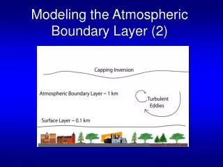
Modeling the Atmospheric Boundary Layer (1)
150 likes | 484 Vues
Modeling the Atmospheric Boundary Layer (1). Review of last lecture. Vertical structure of the atmosphere and definition of the boundary layer Vertical structure of the boundary layer Definition of turbulence and forcings generating turbulence

Modeling the Atmospheric Boundary Layer (1)
E N D
Presentation Transcript
Review of last lecture • Vertical structure of the atmosphere and definition of the boundary layer • Vertical structure of the boundary layer • Definition of turbulence and forcings generating turbulence • Static stability and vertical profile of virtual potential temperature: 3 cases. Richardson number • Boundary layer over ocean • Boundary layer over land: diurnal variation
References • Holton, J. R., 1992: An Introduction to Dynamic Meteorology, Academic Press, Ch 5 • Stull, R. B., 1988: An Introduction to Boundary Layer Meteorology, Springer, Ch 2 • Lappen, C.-L, and D. A. Randall, 2001: Towards a unified parameterization of the boundary layer and moist convection. Part I: A new type of mass-flux model. J. Atmos. Sci., 58, 2021-2036. • Bretherton, C.S., J.R. McCaa, and H. Grenier, 2004: A new parameterization for shallow cumulus convection and its application to marine subtropical cloud-topped boundary layers. Part I: Description and 1-D results. Mon. Wea. Rev., 132, 864-882.
Reynolds averaging (1) Separate mean and turbulent components Assume you are given a time series of zonal wind speed u for a period of one hour, the zonal wind speed can be decomposed into two components: u = U + u’ where U = < u > is the time average (< > means time average, over one hour here) and is called the time mean component, while u’ is the fluctuation around U, i.e. u’ = u - U and is called the turbulent component. (2) Do time average < U > = U < u’ > = 0 < A u’ > = A < u’ > = 0 Only cross terms <a’b’> are left. They are also called non-linear terms.
Intensity of turbulence: Turbulent kinetic energy (TKE) Mean kinetic energy MKE = (U2 + V2 + W2)/2 Turbulent kinetic energy TKE = ‹u’2 + v’2 + w’2 ›/2 ‹ ›represents time average Time evolution (diurnal) Vertical profile
Eddy fluxes The zonal momentum equation is: u/t + uu/x + vu/y + wu/z = - -1p/x + fv Apply Reynolds averaging u= U+u’, v=V+v’, w=W+w’, p=P+p’: (U+u’)/t + (U+u’)(U+u’)/x + (V+v’)(U+u’)/y + (W+w’)(U+u’)/z = - c(P+p’)/x + f(V+v’) The brackets can be expanded to: U/t +u’/t + UU/x +Uu’/x +u’U/x +u’u’/x + VU/y +Vu’/y +v’U/y +v’u’/y + WU/z +Wu’/z +w’U/z +w’u’/z = - -1 P/x - -1 p’/x + fV +fv’ Do time average < > to both sides of the equation. With < A u’> = 0, we can remove many linear eddy terms: <U/t +u’/t + UU/x +Uu’/x +u’U/x +u’u’/x + VU/y +Vu’/y +v’U/y +v’u’/y + WU/z +Wu’/z +w’U/z +w’u’/z> = <- -1 P/x - -1 p’/x + fV +fv’>
Eddy fluxes (cont.) Rearrange the order of the remaining terms, the equation becomes: <U/t +UU/x +VU/y +WU/z +u’u’/x +v’u’/y +w’u’/z> = - -1 P/x + fV With the aid of mass balance u’/x+v’/y+w’/z = 0, we add u’(u’/x+v’/y+w’/z) to the left side of the equation: <U/t +UU/x +VU/y +WU/z +u’u’/x +v’u’/y +w’u’/z +u’u’/x +u’v’/y +u’w’/z> = - -1 P/x + fV By defination D/Dt = /t+u/x+v/y+w/z, and (ab)/x=ab/x+ ba/x, so: DU/Dt +<u’u’>/x +<v’u’>/y +<w’u’>/z = - -1 P/x + fV
Eddy fluxes (cont.) Away from the regions with horizontal inhomogeneities (e.g. shoreline, towns, forest edges), the horizontal eddy fluxes are generally much smaller than the vertical eddy fluxes, and can be neglected: DU/Dt +<u’u’>/x +<v’u’>/y +<w’u’>/z = - -1 P/x + fV Then we have: DU/Dt = - -1 P/x + fV -<w’u’>/z = Fx (force due to turbulent fluxes) <u’w’> is called the eddy zonal momentum flux Derivation is similar for the eddy meridional momentum flux <v’w’>, eddy heat flux <h’w’>, and eddy moisture flux <q’w’>
Vertical profiles of eddy fluxes Day Night
Summary • Reynolds averaging: Separation of mean and turbulent components u = U + u’, < u’ > = 0 • Intensity of turbulence: turbulent kinetic energy (TKE) • Eddy fluxes Fx = - <u’w’>/z TKE = ‹ u’ 2 + v’ 2 + w’ 2 ›/2