Atmospheric General Circulation Modeling
Atmospheric General Circulation Modeling. Anthony J. Broccoli Dept. of Environmental Sciences. Today’s Lecture. Modeling principles Hierarchy of atmospheric models Governing equations for AGCMs Grid vs. spectral Parameterization Using AGCMs to study climatic change. Why Do We Use Models?.

Atmospheric General Circulation Modeling
E N D
Presentation Transcript
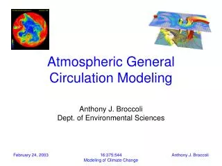
Atmospheric General Circulation Modeling Anthony J. BroccoliDept. of Environmental Sciences 16:375:544Modeling of Climate Change
Today’s Lecture • Modeling principles • Hierarchy of atmospheric models • Governing equations for AGCMs • Grid vs. spectral • Parameterization • Using AGCMs to study climatic change 16:375:544Modeling of Climate Change
Why Do We Use Models? • To gain quantitative insights into the behavior of the Earth system. • A climate model is a mathematical representation of the physical processes that determine climate. • Models are a natural extension of theory. Theory: analytical solutions. Models: numerical solutions 16:375:544Modeling of Climate Change
Models: Complex or Simple? • “…all models are wrong some are useful. Accepting this principle, the job is not so much the search for the true model but to select one model that is appropriate for the problem in hand.” (G. E. P. Box, 1976) • “A useful model is not one that is ‘true’ or ‘realistic’ but one that is parsimonious, plausible and informative.” (M. Feldstein, 1982) 16:375:544Modeling of Climate Change
Models: Complex or Simple? • Models are simplifications of the complexity of nature. • Models should be carefully matched to the problems they attempt to solve. • “As simple as possible, but no simpler.” (A. Einstein, unknown) 16:375:544Modeling of Climate Change
Example: Earth’s Orbit • A very good approximation of the timing of the seasons can be obtained by considering only the gravitational effects of Earth and Sun. • However, effects of other planets (Jupiter and Saturn) are necessary to explain the slow variations in the shape of Earth’s orbit that are responsible for the ice ages. 16:375:544Modeling of Climate Change
Hierarchy of Atmospheric Models Zero-dimensional model of global energy balance: Accounts for exchange of radiation between Earth system and space.Q = incoming solar radiationa = planetary albedo of EarthTP = effective blackbody temperature of Earth-atmosphere systems = Stefan-Boltzmann constant 16:375:544Modeling of Climate Change
Hierarchy of Atmospheric Models One-dimensional models Examples: • Energy balance model (e.g., MAGICC) • Single column model (e.g., radiative-convective model) 16:375:544Modeling of Climate Change
Two-dimensional models Example: Zonally averaged model Express prognostic variables in “primitive equations” as sum of zonal mean and eddy terms. Zonally average the equations. Either set eddies to zero (axially symmetric model), specify them from data, or use some other closure method. Hierarchy of Atmospheric Models 16:375:544Modeling of Climate Change
“Primitive equations” are used in most AGCMs. The following processes are represented: conservation of momentum conservation of thermodynamic energy conservation of mass conservation of water vapor equation of state Governing Equations for AGCMs 16:375:544Modeling of Climate Change
Governing Equations for AGCMs 16:375:544Modeling of Climate Change
Governing Equations for AGCMs momentum eq. 16:375:544Modeling of Climate Change
Governing Equations for AGCMs momentum eq. thermodynamic eq. 16:375:544Modeling of Climate Change
Governing Equations for AGCMs momentum eq. thermodynamic eq. conservation of water vapor 16:375:544Modeling of Climate Change
Governing Equations for AGCMs momentum eq. thermodynamic eq. conservation of water vapor conservation of mass 16:375:544Modeling of Climate Change
Governing Equations for AGCMs momentum eq. thermodynamic eq. conservation of water vapor conservation of mass hydrostatic eq. 16:375:544Modeling of Climate Change
Numerical Methods in AGCMs • Finite difference methods: Derivatives appearing in the governing equations are approximated using differences in dependent variables over finite space and time intervals. Example: First-order centered difference. 16:375:544Modeling of Climate Change
Numerical Methods in AGCMs • Spectral transform method: Use a spherical harmonic basis for horizontal expansion of scalar fields In the spectral transform method, model variables arerepresented by truncated series of spherical harmonics and grid point values. 16:375:544Modeling of Climate Change
Spectral Transform Method Advantages: • Analytic representation of derivatives improves numerical accuracy. • Semi-implicit time differencing implemented easily. • Absence of “pole problem.” 16:375:544Modeling of Climate Change
Spectral Transform Method Disadvantages: • Representation of topography (smoothness, Gibbs ripples). • Computational overhead at high resolution. • Less intuitive mapping onto scalable computer architecture. 16:375:544Modeling of Climate Change
Spectral Truncation Methods R = Rhomboidal T = Triangular B = Both n R5 m 16:375:544Modeling of Climate Change
Spectral Truncation Methods R = Rhomboidal T = Triangular B = Both n T7 m 16:375:544Modeling of Climate Change
Spectral Truncation Methods R = Rhomboidal T = Triangular B = Both n R5 and T7 havesame number ofdegrees of freedom. m 16:375:544Modeling of Climate Change
Governing Equations for AGCMs 16:375:544Modeling of Climate Change
Governing Equations for AGCMs These terms involveprocesses that occuron scales unresolvedby the model. 16:375:544Modeling of Climate Change
Parameterization • Parameterization: The representation of subgrid-scale phenomena as functions of the variables that are represented on the model grid. • Goal is to make parameterizations physical, scale-independent, and nonempirical, but this goal is difficult to achieve. 16:375:544Modeling of Climate Change
What Processes Are Parameterized? • Atmospheric radiative transfer (solar and longwave radiation) • Moist convective processes. • Stable precipitation. • Planetary boundary layer. • Cloud formation and radiative interactions. • Mechanical dissipation of kinetic energy. 16:375:544Modeling of Climate Change
Parameterizations: Achilles’ Heel? • Considerable uncertainties surround physical parametrizations. • Differences in parameterizations are likely responsible for much of the model-dependent behavior in climate change simulations. • In many cases, physical processes are not adequately understood. 16:375:544Modeling of Climate Change
How To Improve Parameterization? • Process studies, including field experiments, single column modeling, etc., can lead to better constraints on physical processes. • Ultimately, increased spatial resolution can allow more processes to be modeled explicitly. (But there are many orders of magnitude between spatial resolution of most advanced global models and spatial scales of cloud formation!) 16:375:544Modeling of Climate Change
Using Atmospheric GCMs To Study Climatic Change • Atmospheric GCMs require a set of lower boundary conditions. • Land surface models are often treated as integral components of atmospheric GCMs. • What to do for oceanic regions? • Specify climatological sea surface temperature (SST). • Specify climatological SST + SST anomalies. 16:375:544Modeling of Climate Change
Experimental design: Prescribe time-varying SSTs (global, tropical Pacific only, etc.) and identify atmospheric response. This experimental design has been widely used, and forms the basis for the Atmospheric Model Intercomparison Project (AMIP) protocol. Atmospheric Response To ENSO Variability 16:375:544Modeling of Climate Change
ENSO Response in Western Pacific Near-surface circulationchanges: El Niño minusLa Niña (courtesy of N.-C. Lau, GFDL) 16:375:544Modeling of Climate Change
Interannual Variations in Water Vapor Temporal variations in tropical-mean precipitable water: Simulated vs. observed(courtesy of B. J. Soden, GFDL) 16:375:544Modeling of Climate Change
Limitations of Prescribing SSTs • Prescribed SST anomaly (i.e., AMIP-type) experiments are most effective when the ocean is primarily forcing the atmosphere. (Tropical surface heating → anomalous convection → atmospheric teleconnection patterns.) • Prescribed SST experiments are also useful in isolating purely internal atmospheric variability (i.e., the variability that would occur even in the absence of external forcing or coupled air-sea interactions) 16:375:544Modeling of Climate Change
Arctic Oscillation In the real world, the positivephase of the AO features anenhanced SLP gradient overthe high-latitude NorthAtlantic Ocean. 16:375:544Modeling of Climate Change
Arctic Oscillation The enhanced westerliesincrease the advection ofcold air across offshore,cooling the sea surface. Over Europe, theonshore flow isstrengthened, whichcauses a warming. 16:375:544Modeling of Climate Change
Simulation of Arctic Oscillation If one were to prescribe theSST pattern that accompanies the positive phase of the AO, would Europe experience positive temperature anomalies? 16:375:544Modeling of Climate Change
Simulation of Arctic Oscillation Probably not! Cooler than normal water upstream would probably lead to negative anomalies over Europe. Why doesn’t the response match the real world? Because the SST anomalies in the real world arise primarily as an oceanic response to atmospheric forcing. 16:375:544Modeling of Climate Change
Limitations of Prescribing SSTs • One may be interested in using a climate model to study processes that will alter the sea surface temperature. • Examples: What is the response of climate to major volcanic eruption? How will increasing greenhouse gases affect future climate? 16:375:544Modeling of Climate Change
Is There a Better Set of Lower Boundary Conditions? • Yes! The lower boundary conditions for the atmosphere could be determined interactively in response to processes internal to the model. • This goal can be achieved by coupling the atmosphere to an ocean model. 16:375:544Modeling of Climate Change


![READ [PDF] The Atmospheric General Circulation](https://cdn7.slideserve.com/12653918/pdf-read-online-the-chemistry-book-from-gunpowder-dt.jpg)