Efficient Global Illumination with Photon Ray Splatting
300 likes | 325 Vues
Learn about photon ray splatting for efficient global illumination, adaptive bandwidth selection, and glossy light field representation. Explore advanced techniques in computer graphics research.

Efficient Global Illumination with Photon Ray Splatting
E N D
Presentation Transcript
EG 2007, 3.9.-7.9. Prague Global Illumination using Photon Ray Splatting Robert Herzog* Vlastimil Havran‡ S. Kinuwaki* K. Myszkowski* H.-P. Seidel* *MPI Informatik ‡Czech Technical University Prague Germany Czech Republic
Motivation: Filling the gap between photon density estimation and final gathering Photon Density Estimation Photon Ray Splatting Low-frequency noise Overestimation at corners Darkening near boundaries Direction undersampling for glossy BRDFs Washed out illumination for high-frequency geometry
Related Work • Ray Maps for Global Illumination, [Havran et al., EGSR 2005] • Gathering of photon rays for a disc in the tangent plane • Eliminates boundary bias • Complex and memory demanding search data structures • Scalable Photon Splatting for Global Illumination, [Lavignotte el al., Graphite 2003] • Efficient image based photon splatting approach with adaptive bandwidth selection • Restricted to triangle meshes and only diffuse light transport towards camera • Path Differentials and Applications, [Suykens et al., EGSR 2001] • Designed for antialiasing and adaptive radiosity tessellation • Radiance Caching for Efficient Global Illumination Computation, [Křivánek et al., IEEE TVCG 2005] • State-of-the-art for (ir)radiance caching on diffuse and glossy surface
Density Estimation Metrics Standard photon density estimation on surfaces [Photon-maps, H.W. Jensen ‘01] Photon density estimation for a disc in the tangent plane [Ray-maps, Havran et al. EGSR ’05] Cosine-weighted photon density estimation in ray-space [Eurographics ’07]
E(x) = L(x,ω) cosθx dσ(ω) E(x) = L(x,ω) cosθx dσ(ω) d2Φ(x,ω) dΦ(x,ω) cosθxdσ(ω) = = d2Φ(x,ω) dA(x) cosθxdσ(ω) dA(x) cosθx = dA┴(x,ω) ΔΦi (xi ,ωi) ΔΦi (xi ,ωi) cosθi Kh(ri) Kh(ri) ΔA┴(x,ωi) ΔA(x) Basic Derivation Irradiance from incident photon rays: ( i.e. use directional information of incident flux ) Irradiance from incident photon hit points:
Ray Splatting instead of Gathering • Efficient gathering of photon rays intersecting a sphere needs complex search data structures (e.g. ray maps [Havran et al. 05]) • Our solution: photon ray splatting instead of gathering • Boils down to search over point data Kh(r)
Choosing the Bandwidth (Splat-radius) • Photon density estimation needs adaptive bandwidth selection • Various statistical methods for bandwidth selection exist – though often too complex to be used for efficient photon density estimation • Common k-nearest-neighbor (k-nn) method is computational intensive • Either costly search for each density estimation query (gathering methods) • Or costly precomputation of the k-nn radius per photon (splatting methods) • Remedy: exploit knowledge from photon sampling, i.e. choose a photon’s splatting radius according to photon path probability density • We get this almost for free !!!
direct light (1 bounce) indirect light (>1 bounces) x0 Photon Path Probability Density Photon path probability: ·g(x0, x1) ·g(xi-1, xi) pe(x0, x1) ps┴(xi-1 , xi , xi+1) p( X ) = pe(x0, x1) ~ Le ·cos(θ0 →1) g(xi, xj) ~ cos(θj←i)/||xi-xj||2 ps┴(xi, xj, xk) ~ fbrdf (xi, xj, xk)·cos(θj→k) θ1 x1 θ2 x2
Adaptive Bandwidth Selection • Choose the photon bandwidth inversely proportional to its path probability density • Reliable estimate only for a small number of bounces (1 to 2) • Need to slightly modify formula to become robust • See paper for details! Color-coded visualization of the bandwidth (shown as photon splats) 2. bounce 4. bounce 1-6 bounces Indirect Illumination
Efficient Nearest Neighbor Search • Nearest neighbor search for ray splatting is simpler than for ray gathering (e.g. ray maps [Havran et al. EGSR05]) • Boils down to a search for point samples in a cylindrical bounding volume • We use a standard kd-tree constructed on top of the eye samples with axis-aligned spatial splitting planes
Search in the Spatial kD-Tree tb R t+ t- ta tb > t- ta< t+ !tb > t- ta< t+ t- leaf R R tb ta Eye sample array Search buffer ,(ta ,t+) stack
Moderately Glossy Surfaces • With ray density estimation we gain more information about the direction of incident flux • since more photons contribute to a surface point • no matter what is the size and orientation of the surface • Means: less noise in the directional domain at grazing angles • However, sampling is view-independent!!! • View-dependent importance sampling of BRDF (future work)
dΦ(x,ω) cosθx Ylm(ω) λlm(x)≈ dA┴(x,ω) Glossy Light Field Representation • We tested 2 different methods for capturing the incident radiance field • Accumulating flux in discrete directional strata (uniformly distributed) • Projecting the incident flux onto a spherical basis (spherical harmonics) (all BRDF data is precomputed in spherical harmonics basis) ΔΦ(θ0,φ0) ΔΦ(θ0,φ0) ΔΦ(θ1,φ1) ΔΦ(θ1,φ1) λlm(x)+= Ylm (θ0,φ0) *Kh(r1) cos(θ1) *Kh(r0) cos(θ0) (θ1,φ1) *Kh(r1) cos(θ1) *Kh(r0) cos(θ0) * s(θ0,φ0) →S0(x) += s(θ1,φ1) →S3(x)+= ΔA┴ ΔA┴ ΔA┴ ΔΦ(θ1,φ1) ΔΦ(θ1,φ1) ΔΦ(θ0,φ0) ΔΦ(θ0,φ0) S3 r0 r1 S0
(Ir)radiance Caching • Computation of (ir)radiance for each pixel is still too slow • However, irradiance function is really smooth due to low-pass filtering via density estimation • sparse sampling of the (ir)radiance is sufficient • We propose an algorithm similar to cache splatting[Gautron et al., EGSR ’05]in the spherical harmonics basis • Cache interpolation gives additional filtering of noisy photon splats reduce overall splat radius more efficient ray splatting
Radiance Cache Splatting Noisy input from ray splatting Adaptive radiance cache splatting BRDF modulated and filtered result
Changes to (Ir)radiance Caching • Due to view-independent ray splatting, we require a multi-pass cache splatting algorithm • For filtering purposes use smooth weighting function (e.g. bi-weight) More than one cache records must contribute to a pixel • Cache density and thus the filtering depends on the geometric gradient estimated using the split-sphere model [Ward ’88] Ward ’88 Bi-weight Estimating harmonic mean distance Rc at cachesr1and r2from projected ray distances (z1,2) to the ray origins (red circle). a·Rc -a·Rc Cache weighting functions
Multi-Pass Radiance Cache Splatting Cache locations (red) + cache weights (~grey shade) Cache splatting result Pass 2 Pass 1 Pass 3
Final gathering (1200 rays per pixel) Photon density estimation (500 k-nn) Ray splatting with caching and filtering Photon ray splatting ~4000 sec 29 sec 35 sec 20 sec Results: Diffuse Sibenik Scene • 500,000 indirect diffuse photons • 512 x 512 image resolution • Compared against reference (photon mapping + final gathering)
10001000 pixel, 200.000 photons 500500 pixel, 500.000 photons 10001000 pixel, 300.000 photons Results K-nn Photon Density Estimation 69 sec (400 k-nn) 66 sec (600 k-nn) 92 sec (400/ 250 k-nn) Photon Ray Splatting (with radiance caching) 64 sec (20 sec) 52 sec 63 sec (16 sec)
Two-Pass Final Gathering Path-traced (2000 rays) Conference Scene 4700700 pixels, 160.000 photons Ray splatting (600 rays) ~ 64 min Photon mapping (70 k-nn 600 rays) ~ 85 min
Conclusions • Ray density estimation as trade-off between photon density estimation and final gathering • No boundary bias, no topological bias • Works well with (ir)radiance caching • However, still problems with proximity bias (light leaking) • requires occlusion testing (future work) (see [Herzog, Pacific Graphics ‘07]) • only low-frequency (indirect) illumination can be rendered so far • More details provided in a technical report (coming soon)
Future Work • Improving adaptive cache splat size computation • Make use of illumination gradients and density estimation variance (estimated from the number of photon splats per cache) to compute a better cache splat size • Temporal domain • Reuse caches for future frames and filter in temporal domain • Detect occlusions during photon ray traversal
Occlusion Testing camera camera Current splatting neglects occlusion in the footprint Correctly masking the density estimation kernel
Unpublished Extensions: What about Occlusion? Ray Splatting Visibility Ray Splatting Lightcuts [Walter 05] (reference) Direct light (50,000 photons/ VPLs) Conference Scene, (1000 x 1000 eye samples) 26 sec 30 sec 675 sec (~245 rays) Global Illumination (250,000 photons/ VPLs) 85 sec 104 sec 1070 sec (~339 rays)
(Additional Material – Not presented at EG ’07)Bandwidth Selection: Practical Issues • Clamp squared distance term in path probability density • Two user parameters to control bandwidth: • Overall noise bias level ( C ) • Variance in bandwidth ( S ), i.e. sensitivity to path probability density (S=0 : constant bandwidth) • For convenience S should be individually chosen for direct and indirect light • Direct light ( S ~ [ 0.5 .. 0.7 ] ) • Indirect light ( S ~ [ 0.1 .. 0.2 ] ) • Bandwidth automatically adapts when number of photons changes • (proportional to 6th root of photon number)
(Additional Material – Not presented at EG ‘07)Cache Weighting Functions := := Ward ‘88 Clampled Ward := Smoothed Ward Biweight := wc(x):= cache weighting function Rc := harmonic mean distance a:= user defined cache-error nc:= cache surface normal n := surface normal at position x -a·Rc a·Rc
(Additional Material – Not presented at EG ‘07)Irradiance Gradients for Ray Splatting Angle θi with surface normal does not change in our metric (ray’s direction is constant) (xi ,ωi) ray.dir r(x,xi,wi) Vx x Ux Kh is the Epanechnikov kernel function.
(Additional Material – Not presented at EG ‘07)Ray Cache Splatting with Irradiance Gradients (i.e. sample denser and thus filter less where the gradient is high) Estimated irradiance gradient magnitude from ray splatting Caveat: use gradient only for determining sampling density, not for cache interpolation!!! (gradients are too noisy) Sharpen shadow boundaries Cache splat result with gradients Cache splat result without gradients Difference image (color coded) Interpolated irradiance (cache splatting for direct + Indirect Light) (300.000 photons) 5.4 sec 5.7 sec
(Additional Material – Not presented at EG ‘07)Scalability of Photon Ray Splatting • Ray splatting only (directly to pixels) (RS direct) • k-NN Photon density estimation (PM k-NN) • Ray splatting to the directional histogram (RS histogram) • Ray splatting + SH radiance caching (RS+SH caching) • Ray splatting time to SH radiance caches (RS only) 500.000 photons 500 x 500 pixels