Lecture 3. ILP (Instruction-Level Parallelism)
COM515 Advanced Computer Architecture. Lecture 3. ILP (Instruction-Level Parallelism). Prof. Taeweon Suh Computer Science Education Korea University. ILP. Fine-grained parallelism All processors since about 1985 use pipelining to overlap the execution of instruction and improve performance


Lecture 3. ILP (Instruction-Level Parallelism)
E N D
Presentation Transcript
COM515 Advanced Computer Architecture Lecture 3. ILP (Instruction-Level Parallelism) Prof. Taeweon Suh Computer Science Education Korea University
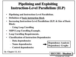
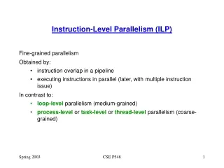
ILP • Fine-grained parallelism • All processors since about 1985 use pipelining to overlap the execution of instruction and improve performance • This potential overlap among instructions is called instruction-level parallelism (ILP), since the instructions can be evaluated in parallel • ILP is a measure of how many of the operations in a computer program can be performed simultaneously - Wikipedia • There are 2 largely separable approaches to exploiting ILP • Hardware-based approach relies on hardware to help discover and exploit parallelism dynamically • Software-based approach relies on software technology (compiler) to find parallelism statically • Limited by • Data dependency • Control dependency
Dependence & Hazard • A hazard is created whenever there is a dependence between instructions, and they are close enough that the overlap during execution would change the order of access to the operand involved in the dependence • Because of the dependence, we must preserve the what it called program order • Data hazard • RAW (Read After Write) or True data dependence • WAW (Write After Write) or Output dependence • WAR (Write After Read) or Antidependence • RAR (Read After Read) is not a hazard
True dependency forces “sequentiality” ILP = 3/3 = 1 ILP Example • False dependency removed • ILP = 3/2 = 1.5 i1: load r2, (r12) i2: add r1, r2, 9 i3: mul r8, r5, r6 c1=i1: load r2, (r12) c2=i2: add r1, r2, 9 c3=i3: mul r2, r5, r6 t t o a c1: load r2, (r12) c2: add r1, r2, #9 mul r8, r5, r6 Prof. Sean Lee’s Slide
Window in Search of ILP R5 = 8(R6) R7 = R5 – R4 R9 = R7 * R7 R15 = 16(R6) R17 = R15 – R14 R19 = R15 * R15 ILP = 1 ILP = ? ILP = 1.5 Prof. Sean Lee’s Slide
Window in Search of ILP R5 = 8(R6) R7 = R5 – R4 R9 = R7 * R7 R15 = 16(R6) R17 = R15 – R14 R19 = R15 * R15 Prof. Sean Lee’s Slide
Window in Search of ILP R5 = 8(R6) R7 = R5 – R4 R9 = R7 * R7 R15 = 16(R6) R17 = R15 – R14 R19 = R15 * R15 C1: C2: C3: • ILP = 6/3 = 2 better than 1 and 1.5 • Larger window gives more opportunities • Who exploit the instruction window? • But what limits the window? Prof. Sean Lee’s Slide
Ambiguous dependency also forces “sequentiality” To increase ILP, needs dynamic memory disambiguation mechanisms that are either safe or recoverable ILP could be 1, could be 3, depending on the actual dependence Memory Dependency i1: load r2, (r12) i2: store r7, 24(r20) i3: store r1, (0xFF00) ? ? ? Prof. Sean Lee’s Slide
ILP, Another Example When only 4 registers available R1 = 8(R0) R3 = R1 – 5 R2 = R1 * R3 24(R0) = R2 R1 = 16(R0) R3 = R1 – 5 R2 = R1 * R3 32(R0) = R2 ILP = Prof. Sean Lee’s Slide
ILP, Another Example When more registers (or register renaming) available R1 = 8(R0) R3 = R1 – 5 R2 = R1 * R3 24(R0) = R2 R5 = 16(R0) R6 = R5 – 5 R7 = R5 * R6 32(R0) = R7 R1 = 8(R0) R3 = R1 – 5 R2 = R1 * R3 24(R0) = R2 R1 = 16(R0) R3 = R1 – 5 R2 = R1 * R3 32(R0) = R2 ILP = Prof. Sean Lee’s Slide
Basic Block • A straight line code sequence with no branches • For typical MIPS programs, the average dynamic branch frequency is often between 15% and 25% • There are only 3 to 6 instructions between a pair of branches • But, these instructions are likely to depend on one another, the amount of overlap within a basic block is likely to be less than the average basic block size • To obtain substantial performance enhancements, we must exploit ILP across multiple basic blocks
i1: lw r1, (r11) i2: lw r2, (r12) i3: lw r3, (r13) i4: add r2, r2, r3 i5: bge r2, r9, i9 i6: addi r1, r1, 1 i7: mul r3, r3, 5 i8: j i4 i9: sw r1, (r11) i10: sw r2, (r12) I11: jr r31 Basic Blocks a = array[i]; b = array[j]; c = array[k]; d = b + c; while (d<t) { a++; c *= 5; d = b + c; } array[i] = a; array[j] = d; Prof. Sean Lee’s Slide
Basic Blocks a = array[i]; b = array[j]; c = array[k]; d = b + c; while (d<t) { a++; c *= 5; d = b + c; } array[i] = a; array[j] = d; i1: lw r1, (r11) i2: lw r2, (r12) i3: lw r3, (r13) i4: add r2, r2, r3 i5: bge r2, r9, i9 i6: addi r1, r1, 1 i7: mul r3, r3, 5 i8: j i4 i9: sw r1, (r11) i10: sw r2, (r12) I11: jr r31 Prof. Sean Lee’s Slide
BB1 BB2 BB3 BB4 Control Flow Graph i1: lw r1, (r11) i2: lw r2, (r12) i3: lw r3, (r13) i4: add r2, r2, r3 i5: jge r2, r9, i9 i6: addi r1, r1, 1 i7: mul r3, r3, 5 i8: j i4 i9: sw r1, (r11) i10: sw r2, (r12) I11: jr r31 Prof. Sean Lee’s Slide
lw r1, (r11) lw r2, (r12) lw r3, (r13) add r2, r2, r3 jge r2, r9, i9 sw r1, (r11) jr r31 sw r2, (r12) addi r1, r1, 1 mul r3, r3, 5 j i4 ILP (without Speculation) BB1 = 3 BB1 i1: lw r1, (r11) i2: lw r2, (r12) i3: lw r3, (r13) BB2 = 1 BB3 = 3 BB2 i4: add r2, r2, r3 i5: jge r2, r9, i9 BB4 = 1.5 BB1 BB2 BB3 BB3 BB4 ILP = 8/4 = 2 i6: addi r1, r1, 1 i7: mul r3, r3, 5 i8: j i4 i9: sw r1, (r11) i10: sw r2, (r12) I11: jr r31 BB1 BB2 BB4 ILP = 8/5 = 1.6 Modified from Prof. Sean Lee’s Slide
lw r1, (r11) lw r2, (r12) lw r3, (r13) add r2, r2, r3 addi r1, r1, 1 mul r3, r3, 5 j i4 jge r2, r9, i9 lw r1, (r11) lw r2, (r12) lw r3, (r13) add r2, r2, r3 sw r1, (r11) jge r2, r9, i9 sw r2, (r12) jr r31 ILP (with Speculation, No Control Dependence) BB1 BB2 BB3 BB1 i1: lw r1, (r11) i2: lw r2, (r12) i3: lw r3, (r13) ILP = 8/3 = 2.67 BB2 BB1 BB2 BB4 i4: add r2, r2, r3 i5: jge r2, r9, i9 ILP = 8/3 = 2.67 BB3 BB4 i6: addi r1, r1, 1 i7: mul r3, r3, 5 i8: j i4 i9: sw r1, (r11) i10: sw r2, (r12) I11: jr r31 Prof. Sean Lee’s Slide
Flynn’s Bottleneck • ILP 1.86 • Programs on IBM 7090 • ILP exploited within basic blocks • [Riseman & Foster’72] • Breaking control dependency • A perfect machine model • Benchmark includes numerical programs, assembler and compiler BB0 BB1 BB2 BB4 BB3 Modified from Prof. Sean Lee’s Slide
David Wall (DEC) 1993 • Evaluating effects of microarchitecture on ILP • OOO with 2K instruction window, 64-wide, unit operation latency • Peephole alias analysis (alias by instruction inspection) inspecting instructions to see if any obvious independence between addresses • Indirect jump predict • Ring buffer (for procedure return): similar to return address stack • Table: last time prediction Modified from Prof. Sean Lee’s Slide
arg locals return addr return val sp=sp-48 Stack Pointer Impact • Stack Pointer register dependency • True dependency upon each function call • Side effect of language abstraction • See execution profiles in the paper • “Parallelism at a distance” • Example: printf() • One form of Thread-level parallelism old sp Stack in memory Modified from Prof. Sean Lee’s Slide
Removing Stack Pointer Dependency [Postiff’98] $sp effect Prof. Sean Lee’s Slide
Many embedded system designers chose this Exploiting ILP • Hardware • Control speculation (control) • Dynamic Scheduling (data) • Register Renaming (data) • Dynamic memory disambiguation (data) • Software • (Sophisticated) program analysis • Predication or conditional instruction (control) • Better register allocation (data) • Memory Disambiguation by compiler (data) Prof. Sean Lee’s Slide
Other Parallelisms SIMD (Single instruction, Multiple data) • Each register as a collection of smaller data Vector processing • e.g. VECTOR ADD: add long streams of data • Good for very regular code containing long vectors • Bad for irregular codes and short vectors Multithreading and Multiprocessing (or Multi-core) • Cycle interleaving • Block interleaving • High performance embedded’s option (e.g., packet processing) Simultaneous Multithreading (SMT): Hyper-threading • Separate contexts, shared other microarchitecture modules Prof. Sean Lee’s Slide