8-1 Introduction
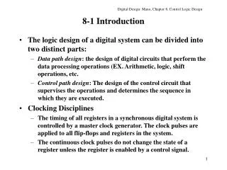
8-1 Introduction. The logic design of a digital system can be divided into two distinct parts: Data path design : the design of digital circuits that perform the data processing operations (EX. Arithmetic, logic, shift operations, etc.

8-1 Introduction
E N D
Presentation Transcript
8-1 Introduction • The logic design of a digital system can be divided into two distinct parts: • Data path design: the design of digital circuits that perform the data processing operations (EX. Arithmetic, logic, shift operations, etc. • Control path design: The design of the control circuit that supervises the operations and determines the sequence in which they are executed. • Clocking Disciplines • The timing of all registers in a synchronous digital system is controlled by a master clock generator. The clock pulses are applied to all flip-flops and registers in the system. • The continuous clock pulses do not change the state of a register unless the register is enabled by a control signal.
Control and data processor (Fig. 8-1) • The control logic that generates the signals for sequencing the operations in the data processor is essentially a sequential machine. (Mealy machine) • Next state = F(current state, external inputs, status conditions) • Output= G (current state, external inputs, status conditions) • Control organization • Two major types of control organization • Hardwired control: The control logic is implemented with gates and flip-flops similar to a sequential circuit. • Advantage: Fast mode of operation • Disadvantage: Require changes in the wring among various components if the design has to be modified.
Microprogrammed control: The control information such as control functions or control words are stored as 1’s and 0’s is a special memory. • Advantage: Any changes or modifications can be done merely by changing the contents of the memory. • Disadvantage: Slow mode of operation
8-2 Microprogrammed Control • The purpose of the control unit in a digital system is to initiate a series of sequential steps of operations. At any given time, some operations are to be initiated while others remain idle. • The control variables at any given time can be represented by a string of 1’s and 0’s called a control word. So the control words can be programmed to initiate the various components in the data processor. • A control unit whose binary control variables are stored in a memory is called a microprogrammed control unit. • Each word in control memory is called a microinstruction.
A sequence of microinstructions constitute the microprogram. • The control memory can be a ROM. • By reading the content of the word in ROM at a given address specified the microoperations for the data processor. • Dynamic microprogramming: A microprogram to be loaded initially from the computer console or from magnetic disks. • Generation configuration of a microprogrammed control (Fig. 8-2) • Control address register: Specifies the address of the microinstruction. • Control data register: Holds the microinstruction read from memory.
The location of the next microinstruction is generated by the sequencer. The location may be the next one in sequence, or it may be located elsewhere in the control memory. Some bit of the present microinstruction are used to generate the address of the next microinstruction. • Typical functions of a microprogrammed sequencer • Increment the control address register (CAR) by one. (CAR CAR + 1) • Load into the CAR an address from control memory. (CAR CDR) • Transfer an external address into CAR. (CAR External Input) • Load an initial address into CAR to start the control operations. (CAR Initial address)
Control data register • Data register is sometimes called a pipeline register. • It allows the microoperations specified by the control word to be executed simultaneously with the generation of the next microinstruction, that is, the CAR can be loaded with the address of next microinstruction while the current microinstruction is executing. • This configuration requires a two phase clock, with one phase applied to the address register (CAR) and the other to the control data register. (Fig. XX) • Without control data register • The system can operate without the control data register by applying a single phase clock to the address register. • The CAR can not load a new address while the current microinstruction is executing. (Fig. XX) • For our example we will not use the control data register.
8-3 Control of Processor Unit • Microprogrammed control (Fig. 8-3) • Operation of control unit • CAR receives a new address at any given clock pulse transition. • The 26-bit microinstruction is read. • The control word specifies a microoperation and MUX1 and MUX2 determine the next operation for CAR. • The next transition of the clock transfers the result of the microoperation into destination register, updates the required status bits, and put a new address into the CAR. • Encoding of microinstructions • Microinstruction format(Table 8-1) • Encoding of ALU operations • Encoding of Shifter operations • Encoding of Select input to MUX2
Examples of microinstructions (Table 8-5) Address 36: R1 R1 R2, CAR CAR + 1 Address 40: R3 R3 - 1, CAR 43 Address 52: R4 0, if (S=1) then (CAR 37) else (CAR CAR + 1) Address 56: R5 shl R5, if (C=0) then (CAR 62) else (CAR CAR + 1) Address 59: R2 R6 + R7, CAR External Address
8-4 Microprogram Examples • Example 1: Perform the following operations: 1. R3 R1 - R2 /* This updates C and Z flags */ 2. If R1 < R2 (detected by C=0) then R4 R4 + R1 If R1 > R2 (detected by C=1 and Z=0) then R4 R4 + R2 If R1 = R2 (detected by Z=1) then R4 R4 + 1 3. Output R4 and branch to external address X-Y=X-Y+2n-2n=X+(2n-Y-1)+1-2n=X+Y’+1-2n If X-Y<0 ==> X+Y’+1-2n<0 ==> X+Y’+1<2n ==> No carry If X-Y >= 0 ==> X+Y’+1 >= 2n ==> with carry • Register transfer statement (Table 8-6) • Symbolic microprogram (Table 8-7) • Binary microprogram (Table 8-8)
Example 2: Counting the number of 1’s • Problem: Count the number of 1’s stored in register R1 and set register R2 to that number. • For example, if R1=00110110 then R2=00000100 • Flowchart (Fig. 8-4) • Microprogram (Table 8-9) • The microprogram method is sometimes referred to as firmware.
8.5 Design Example: Binary Multiplier by Hardwired Control • The microprogram is too expensive for the design of small digital systems and not fast enough for high speed computers. • The hardwired control is essentially a sequential circuit whose state at any given time determines the microoperations to be executed in the data processor subsystem. • A multiplier = data processor + control unit
Design of binary multiplier data processor • Example 23 10111 Multiplicand 19 10011 Multiplier -------------------------------------------------------- 10111 10111 Shifted multiplicand 00000 00000 10111 ---------------------------------------------------- 437 110110101 Product • The product of multiplying two n-bit numbers can have up to 2n bits
Shift-And-Add multiplier 10111 Multiplicand 10011 Multiplier --------- 00000 Initial partial product 10111 Shifted multiplicand (SM) --------- 10111 Partial product (PP) 10111 SM --------- 1000101 PP 0000000 SM ------------ 1000101 PP 00000 SM -------------- 01000101 PP 10111 SM ---------------- 110110101 Product • We will shift the partial product instead of multiplicand. • If the corresponding bit in the multiplier is 0, no need to add all 0’s to the partial product.
Register configuration for the multiplier (Fig. 8-5) • n is the number of bits for the multiplier. • The counter P is loaded with the value n before multiplication starts. • Flowchart for binary multiplier (Fig. 8-6) • Required registers • The type of registers needed for the data processor can be derived from the microoperations listed in the flowchart: • Register A must be a shift register with parallel load. • Register Q is a shift register. • Register B is a register with parallel load, • Counter P is a binary count-down counter with parallel load. • Flip-flop C should have a synchronous reset. • Numerical example for binary multiplier (Table 8-10)
8-6 Hardwired Control for Multiplier • The design of a hardwired control is a sequential circuit design problem. • The state diagram of the control circuit. (Fig. 8-7) • Inputs: S, Z, and Q • Outputs: T0, T1, T2, T3 and L • The control logic has two inputs Z and S and four outputs, T0, T1, T2, T3 . • Hardwired control by sequence register(state memory) and decoder • Use a register to sequence the control states and a decoder to provide an output for each state. • An n-bit sequence register is essentially a circuit with n flip-flops together with the associated gates that effect their state transitions.
The control state diagram for binary multiplier has four states and two inputs. We need two flip-flops for the register and a 2-to-4 line decoder. • State table (Transition/excitation and output table) (Table 8-11) • Excitation equations DG0 = D0 = D1’ G0’ S + G1 G0’ = T0 S + T2 DG1 = D1 = G1’ G0 +G1 G0’ + G1 G0 Z’ = T1 +T2 +T3 Z • Logic diagram of the control logic (Fig. 8-9) • Hardwired control by on flip-flop per state • Use one flip-flop per state. We need four flip-flops but no decoder. Only one flip-flop is set to 1 at any particular time; all others are set to 0. • One advantage of this method is the simplicity with which it can be designed. This type of controller can be designed directly by inspection from the state diagram.
Excitation equations DT0=T0 S’ + T3 Z DT1= T0 S DT2= T1 + T3 Z’ DT3= T2 • Sometimes, the one flip-flop per state controller is implemented with a register that has common asynchronous input for resetting all flip-flops initially to 0. Dt0 is modified as follows: DT0=T0 S’ + T3 Z + T0’ T1’ T2’ T3’ • Logic diagram for one flip-flop per state controller
8-7 Example of a Simple Computer • The user of a computer can control the process of operations by means of a program. • A program is a set of instructions that specifies the operations, operands, and the sequence in which processing is to occur. • The data processing task may be altered by specifying a new program with different instructions or by specifying the same instructions with different data. • The instruction codes, together with data are stored in memory. The control reads each instruction from memory and places it in a control register (instruction register). The control then interprets the instruction and proceeds to execute it by issuing a sequence of microoperations. • The ability to store and execute instructions is the most important property of the general purpose computer (i.e., Stored program concept)
Instruction code • An instruction code is a group of bits that instructs the computer to perform a specific operation. • It is usually divided into parts, each having its own particular interpretation (Opcode + Operands). • The most basic part of an instruction code is its operation part (Opcode). • The operation code of an instruction is a group of bits that defines an operation, such as add, subtract, shift, …. • Operation code (Opcode) • The number of bits required for the operation code of an instruction is a function of the total number of operations used. • n bits can specified up to 2n operations.
Operand • An instruction code must specify not only the operation but also the registers or memory words where the operands are to be found. • Two ways of specifying an operand • An operand is said to be specified explicitly if the instruction code contains special bits for its identification. For example, memory address may be specified explicitly as an operand. • An operand is said to be specified implicitly if it is included as part of the definition of the operation. For example, an operation that complements a register in the operation part of the code. • Instruction code format • The format of an instruction is usually depicted in a rectangular box symbolizing the bits of the instruction as they appear in memory word or in a control register • Example of an instruction format (Fig. 8-11) • Numerical example (Fig. 8-12)
Instruction, Operation, and microoperation • An operation is specified by an instruction stored in computer memory. • The operation code bits are interpreted by the control unit as a sequence of control functions to perform the required microoperations for the execution of the instruction. • Block diagram of a simple computer (Fig. 8-13) • Registers (Table 8-12) • The accumulator register (AC) is a general purpose register where the data processing is done. • Instructions (Table 8-13) • 8-bit Opcode specifies 256 instructions, but only six instructions are used here. • Instruction length is defined by the number of bits used by Opcode and operands.
A simple program to perform 83-(52+25) LDI 52 Load 52 into the AC ADI 25 Add 25 to the AC CMA Complement the AC INA Increment the AC ADI 83 Add 83 to the AC STA 250 Store the contents of the AC in M[250]
8-8 Design of a Simple Computer • Instruction execution cycle • Instruction fetch phase --> Instruction execution phases --> Instruction fetch phase …. • Instruction fetch phase: common to all instructions. • It fetches the operation code from memory abnd places it in a control register. • Timing variables T0 and T1 of the timing decoder are used as control functions for the fetch phase. T0: DR M[PC] T1: IR DR, PC PC + 1 • Instruction execution phase • For INA instruction D1T2: AC AC + 1, TC 0
TC 0 implies that control goes back to timing variable T0 to start the fetch phase and read the operation code of the next instruction. • For LDI OPRD instruction D3T2: DR M[PC] D3T3: AC DR, PC PC + 1, TC 0 • For LAD ADRS instruction D5T2: DR M[PC] D5T3: AR DR, PC PC + 1 D5T4: DR M[AR] D5T5: AC DR, TC 0 • Microoperation sequence for the simple computer (Fig. 8-14)
Control Logic • The design of the control logic starts from listing the set of microoperations and control functions. • The list of microoperations specifies the type of registers and associated digital functions that must be incorporated into the data processing part of the system. • The list of control functions specifies the logic gates required for the control unit. • First, scan the register transfer statements and retrieve all these statements that perform the same microoperation. For example, from Fig. 8-14, inspect PC PC + 1, we get • T1+(D3+D4+D5+D6)T3: PC PC + 1. • The associated hardware implementation (Fig. 8-15) • The list of control variables for microoperations (Table 8-14)
The microoperations of the AC C4: AC AC + 1 C5: AC AC’ C6: AC DR C7: AC AC + DR • The hardware design of the simple computer (Fig. 8-10)
Final Project • Department of Computer Engineering and Science, Yuan-Ze University • Course Name: Logic Design • Date out: June 4 • Date due: June 28 • Problem Description • Modify the simple computer described in Chapter 8 to include the following instructions: • BZ branch if Z=1 • BNZ branch if Z=0 • BC branch if C=1 • BNC branch if C=0 • BM branch if S=1 • BP branch if S=0 • BV branch if S=1 • BNV branch if S=0 • JMPI Internally jump (the target address of the above branch and comes from DR) • JMPE Externally jump (the target address comes from outside) • (all branch and jump instructions have an 8-bit absolute target address)
SUBI OPRD Subtract immediate operand AC<--- AC-OPRD • AND OPRD Logical AND AC <--- AC AND OPRD • OR OPRD Logical OR AC<-- AC OR OPRD • XOR OPRD Logical exclusive OR AC<-- AC XOR OPRD • XNR OPRD Logic exclusive NOR AC<--- AC XNR OPRD • NOP No operation PC<--- PC + 1 • TEST OPRD Test (AC is not changed) AC - OPRD • You have at least to add two input signals as follows: • START: Start executing a program when START changes from zero to 1. Once a program starts to execute, START must be set to 0. • RESET: Reset the computer to initial state when it changes from 0 to 1 and remain at least 3 consecutive cycles at 1. Once the computer is reset, this signal must be set to 0. • You must have at least have the following output signals: • BUSY: It is 1 if a program is executing. • PCC_8: 8-bits output to show the value of program counter. • ACC_8: 8-bit output to show the value of accumulator. • SZVC_4: 4-bit output to show the value of status bits. • You are allowed to add more input and output signals as necessary.
The following table shows how the execution of an instruction sets the status bit OPcode Z S C V 00000001 INA Y Y Y Y 00000010 CMA Y Y N N 00000011 LDI Y Y N N 00000100 ADI Y Y Y Y 00000101 SUBI Y Y Y Y 00000110 LDA N N N N 00000111 STA N N N N 00001000 BZ N N N N 00001001 BNZ N N N N 00001010 BC N N N N 00001011 BNC N N N N 00001100 BM N N N N 00001101 BP N N N N 00001110 BV N N N N 00001111 BNV N N N N 00010000 JMPI N N N N 00010001 JMPE N N N N 00010010 AND Y Y N N 00010011 OR Y Y N N 00010100 XOR Y Y N N 00010101 XNR Y Y N N 00010110 NOP N N N N 00010111 TEST Y Y Y Y
Each Team consists of at most two members • Use VHDL to implement such a computer. • Write a program to sort the following data segment that locates at the memory address 240. Store the data in ascending order starting at 240. You must make your program size less than 240 bytes. So you are allowed to use any sorting algorithm that can achieve this goal. • Data segment Address Content 240 35 241 67 242 35 243 108 244 7 245 230 246 56 247 78 248 34 249 121