Probability
E N D
Presentation Transcript
Probability • Probability is fundamental to scientific inference • Deterministic vs. Probabilistic systems • When the knowledge of a system is incomplete, the behavior of the system is not perfectly predictable • Events appear to occur randomly following a probability structure
Definitions • Sample Space - S • Set of all possible events • Coin flip (H,T) • Roll a die (1,2,3,4,5,6) • Exam score (1,2,3,…,100) • Trial • One sample or experiment yielding an observation • Coin flip, dice roll, one exam score
Definitions (cont) • Operations • A and B are two events in S that could occur on any given trial • ~A (Not A) -> A does not occur • AB (union) -> Either A or B occurs • A,B (intersection) -> Both A and B occur • A\B (=A,~B) -> A occurs and B does not
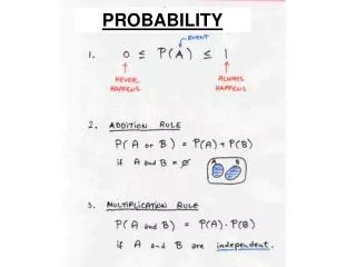
Definitions (cont) • Exhaustive events • AB = S • Ex: Coin flip… HT = S • Exclusive events • A,B= • Ex: Heads and Tails can never occur together • p(A) ≥ 0 • p(S) = 1 • p(AB) = p(A)+ p(B) - p(A,B)
Conditional Probability • Probability that an event (B) will occur given that another event has already occurred (A) • Ex: Probability of lung cancer (unconditional) • Ex: Probability of lung cancer given that you are a smoker (conditional) • p(B|A) = p(B,A) / p(A)
Conditional Probability • Example: - Deck of cards • 52 cards, 4 suites with 13 cards in each suite • p(ace) = 4/52 (unconditional) • p(B-ace|A-ace) - Assume no replacement • p(B,A) = 12 / 2652 • possible pairs of aces / all possible pairs • p(B|A) = (12/2652)/(4/52) = 3/51
Joint Probability • Intersection of two events - p(A,B) • Probability of A and B • Can be viewed as a function of a conditional and an unconditional probability • p(A,B) = p(B|A) p(A) • probability of A times the probability of B given that A has occurred
Joint Probability • Multiplication Rule • Generalizes joint probability to more than 2 events • p(A1,A2,A3…An) = p(A1)*p(A2|A1)*p(A3|A1,A2)*p(An|A1,A2,…,An-1)
Bayes theorem • Conceptually challenging but mathematically simple • Frequentist vs subjective probability views of probability • # of expected occurrences for a set of trials • Degree of belief • Bayes Rule may be viewed as a way to update belief or subjective probability, p(A), as evidence comes in, p(A|B)
Bayes Theorem • p(A|B) = p(A,B)/p(B) • or = p(B|A)p(A)/p(B) • or = p(B|A)p(A)/(p(B|A)p(A)+p(B|~A)p(~A)) • p(A) = Prior Belief • P(A|B) = Posterior belief
Bayes Rule - Example • Morris code • Dots and dashes occur in proportion of 3:4 • Sometimes sent dots (D) aren’t received as dots • Assume p(error) = 1/8 • D = a dot was sent • R = a dot was received • p(D) = 3/7; Probability a dot is sent • 3 times out of 7 a dot is sent • Question: If a dot is received, what is the probability that a dot was sent?
Bayes Rule - Example • p(D|R)? • p(D|R) = p(R|D)p(D)/p(R) • p(D) = 3/7 • p(R|D) = 7/8 • p(R) = ? • p(R) = p(R|D)p(D)+p(R|~D)p(~D) • p(R) = (7/8)(3/7) + (1/8)(4/7) = 25/56 • p(D|R) = (7/8)(3/7)/(25/56)=(21/25)= .84
Independence • Following Bayes Rule, two events are independent if the occurrence of event B doesn’t alter the probability of event A • p(A) = p(A|B) • p(A,B) = p(A) p(B)
Conditional Independence • 2 events, A and B, are independent given C if: • p(A,B|C) = p(A|C) p(B|C)
Discrete Random Variables • A variable that take on a finite number of states with a given probability structure • Ex: faces of a die • Our focus is on discrete random variables with two states • Ex: right/wrong or agree/disagree
Discrete Random Variables • Bernoulli trial • An observation where a random variable may take on only one of two states (yes/no) • Probability Mass Function
Discrete Random Variables • Binomial Distribution • Xi is a binary random variable representing n independent Bernoulli trials each having the same probability (p) of observing a success • Gives the probability of x successes in n trials
Discrete Random Variables • Binomial Probability Mass Function • Ex: n = 3
Discrete Random Variables • X~Bin(n,p) • n & p specify the parameters of a specific binomial distribution • Cumulative Distribution Function (c.d.f.) • FX(x) = P(X ≤ x)=Σpj
Discrete Random Variables Graphic cdf
Continuous Random Variables • Normal distribution- Probability Density Function • X~N(μ,σ)
Normal Distribution • Cumulative Distribution Function
Normal Probability in R • Sampling from a given distribution • X<-rnorm(400,mean=3,sd=3) • hist(x) • Determining the cdf up to a given value • pnorm(0) • pnorm(1.2) • x <- seq(-4,4,by=.1) • y <- pnorm(x) • plot(x,y)
Binomial Probability in R • Distribution function • > x <- seq(0,50,by=1) • > y <- dbinom(x,50,0.2) • > plot(x,y) • > y <- dbinom(x,50,0.6) • > plot(x,y) • > x <- seq(0,100,by=1) • > y <- dbinom(x,100,0.6) • > plot(x,y)
Binomial Probability in R • Cumulative Probability Distribution • > pbinom(24,50,0.5) [1] 0.4438624 • > pbinom(25,50,0.5) [1] 0.5561376 • > pbinom(25,51,0.5) [1] 0.5 • > pbinom(26,51,0.5) [1] 0.610116 • > pbinom(25,50,0.5) [1] 0.5561376 • > pbinom(25,50,0.25) [1] 0.999962 • > pbinom(25,500,0.25) [1] 4.955658e-33
Binomial Probability in R • Sampling • > rbinom(5,100,.2) • [1] 30 23 21 19 18 • > rbinom(5,100,.7) • [1] 66 66 58 68 63 >
