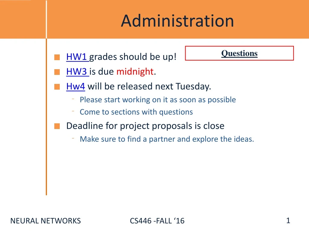
1. Administration Questions • HW1 grades should be up! • HW3 is due midnight. • Hw4will be released next Tuesday. • Please start working on it as soon as possible • Come to sections with questions • Deadline for project proposals is close • Make sure to find a partner and explore the ideas.

2. Recap: Multi-Layer Perceptrons • Multi-layer network • A global approximator • Different rules for training it • The Back-propagation • Forward step • Back propagation of errors • Congrats! Now you know the hardest concept about neural networks! • Today: • Convolutional Neural Networks • Recurrent Neural Networks Output activation Hidden Input

3. Receptive Fields • The receptive field of an individual sensory neuron is the particular region of the sensory space (e.g., the body surface, or the retina) in which a stimulus will trigger the firing of that neuron. • In the auditory system, receptive fields can correspond to volumes in auditory space • Designing “proper” receptive fields for the input Neurons is a significant challenge. • Consider a task with image inputs • Receptive fields should give expressive features from the raw input to the system • How would you design the receptive fields for this problem?

4. A fully connected layer: • Example: • 100x100 images • 1000 units in the input • Problems: • 10^7 edges! • Spatial correlations lost! • Variables sized inputs. Slide Credit: Marc'AurelioRanzato

5. Consider a task with image inputs: • A locally connected layer: • Example: • 100x100 images • 1000 units in the input • Filter size: 10x10 • Local correlations preserved! • Problems: • 10^5 edges • This parameterization is good when input image is registered (e.g., face recognition). • Variable sized inputs, again. Slide Credit: Marc'AurelioRanzato

6. Convolutional Layer • A solution: • Filters to capture different patterns in the input space. • Share parameters across different locations (assuming input is stationary) • Convolutions with learned filters • Filters will be learned during training. • The issue of variable-sized inputs will be resolved with a pooling layer. So what is a convolution? Slide Credit: Marc'AurelioRanzato

7. Convolution Operator • Convolution operator: • takes two functions and gives another function • One dimension: “Convolution” is very similar to “cross-correlation”, except that in convolution one of the functions is flipped. Exampleconvolution:

8. Convolution Operator (2) • Convolution in two dimension: • The same idea: flip one matrix and slide it on the other matrix • Example: Sharpen kernel: Try other kernels: http://setosa.io/ev/image-kernels/

9. Convolution Operator (3) • Convolution in two dimension: • The same idea: flip one matrix and slide it on the other matrix Slide Credit: Marc'AurelioRanzato

10. Complexity of Convolution • Complexity of convolution operator is , for inputs. • Uses Fast-Fourier-Transform (FFT) • For two-dimension, each convolution takes time, where the size of input is . Slide Credit: Marc'AurelioRanzato

11. Convolutional Layer • The convolution of the input (vector/matrix) with weights (vector/matrix) results in a response vector/matrix. • We can have multiple filters in each convolutional layer, each producing an output. • If it is an intermediate layer, it can have multiple inputs! Convolutional Layer Filter Filter Filter Filter One can add nonlinearity at the output of convolutional layer

12. Pooling Layer • How to handle variable sized inputs? • A layer which reduces inputs of different size, to a fixed size. • Pooling Slide Credit: Marc'AurelioRanzato

13. Pooling Layer • How to handle variable sized inputs? • A layer which reduces inputs of different size, to a fixed size. • Pooling • Different variations • Max pooling • Average pooling • L2-pooling • etc

14. Convolutional Nets • One stage structure: • Whole system: Convol. Pooling Fully Connected Layer Stage 1 Stage 2 Stage 3 Input Image Class Label An example system (LeNet): Slide Credit: DruvBhatra

15. Training a ConvNet • The same procedure from Back-propagation applies here. • Remember in backprop we started from the error terms in the last stage, and passed them back to the previous layers, one by one. • Back-prop for the pooling layer: • Consider, for example, the case of “max” pooling. • This layer only routes the gradient to the input that has the highest value in the forward pass. • Hence, during the forward pass of a pooling layer it is common to keep track of the index of the max activation (sometimes also called the switches) so that gradient routing is efficient during backpropagation. • Therefore we have: Convol. Pooling Input Image Class Label Stage 3 Fully Connected Layer Stage 2 Stage 1

16. Training a ConvNet We derive the update rules for a 1D convolution, but the idea is the same for bigger dimensions. • Back-prop for the convolutional layer: The convolution Convol. Pooling A differentiable nonlinearity Now we have everything in this layer to update the filter Input Image Class Label Stage 3 Fully Connected Layer Now we can repeat this for each stage of ConvNet. We need to pass the gradient to the previous layer Stage 2 Stage 1

17. Convolutional Nets Fully Connected Layer Stage 1 Stage 2 Stage 3 Input Image Class Label An example system : Feature visualization of convolutional net trained on ImageNet from [Zeiler & Fergus 2013]

18. ConvNet roots • Fukushima, 1980sdesigned network with same basic structure but did not train by backpropagation. • The first successful applications of Convolutional Networksby Yann LeCun in 1990's(LeNet) • Was used to read zip codes, digits, etc. • Many variants nowadays, but the core idea is the same • Example: a system developed in Google (GoogLeNet) • Compute different filters • Compose one big vector from all of them • Layer this iteratively Demo! See more: http://arxiv.org/pdf/1409.4842v1.pdf

19. Depth matters Slide from [Kaiming He 2015]

20. Practical Tips • Before large scale experiments, test on a small subset of the data and check the error should go to zero. • Overfitting on small training • Visualize features (feature maps need to be uncorrelated) and have high variance • Bad training: many hidden units ignore the input and/or exhibit strong correlations. Figure Credit: Marc'AurelioRanzato

21. Debugging • Training diverges: • Learning rate may be too large → decrease learning rate • BackProp is buggy → numerical gradient checking • Loss is minimized but accuracy is low • Check loss function: Is it appropriate for the task you want to solve? Does it have degenerate solutions? • NN is underperforming / under-fitting • Compute number of parameters → if too small, make network larger • NN is too slow • Compute number of parameters → Use distributed framework, use GPU, make network smaller Many of these points apply to many machine learning models, no just neural networks.

22. CNN for vector inputs • Let’s study another variant of CNN for language • Example: sentence classification (say spam or not spam) • First step: represent each word with a vector in This is not a spam Concatenate the vectors • Now we can assume that the input to the system is a vector • Where the input sentence has length ( in our example ) • Each word vector’s length ( in our example ) OOOOOOO OOOOOOO OOOOOOO OOOOOOO OOOOOOO O OOOOOOOOOOOOOOOOOOOOOOOOOOOOOOOOOO

23. Convolutional Layer on vectors • Think about a single convolutional layer • A bunch of vector filters • Each defined in • Where is the number of the words the filter covers • Size of the word vector • Find its (modified) convolution with the input vector • Result of the convolution with the filter • Convolution with a filter that spans 2 words, is operating on all of the bi-grams (vectors of two consecutive word, concatenated): “this is”, “is not”, “not a”, “a spam”. • Regardless of whether it is grammatical (not appealing linguistically) O OOOOOOOOOOOOO O OOOOOOOOOOOOOOOOOOOOOOOOOOOOOOOOOO A convolutional layer O OOOOOOOOOOOOO O OOOOOOOOOOOOOOOOOOOOOOOOOOOOOOOOOO O OOOOOOOOOOOOO O OOO O OOOOOOOOOOOOOOOOOOOOOOOOOOOOOOOOOO O OOOOOOOOOOOOO O OOOOOOOOOOOOO O OOOOOOOOOOOOOOOOOOOOOOOOOOOOOOOOOO O OOOOOOOOOOOOOOOOOOOOOOOOOOOOOOOOOO

24. Convolutional Layer on vectors • This is not a spam Get word vectors for each words OOOOOOO OOOOOOO OOOOOOO OOOOOOO OOOOOOO Concatenate vectors O OOOOOOOOOOOOOOOOOOOOOOOOOOOOOOOOOO * Perform convolution with each filter O OOOOOO O OOOOOOOOOOOOO Filter bank O OOOOOOOOOOOOO O OOOOOOOOOOOOOOOOOOOO O OOOOOOOOOOOOOOOOOOOO How are we going to handle the variable sized response vectors? Pooling! O OOOO Set of response vectors O OOO #of filters O OOO O OO O OO #words - #length of filter + 1

25. Convolutional Layer on vectors • This is not a spam Get word vectors for each words • Now we can pass the fixed-sized vector to a logistic unit (softmax), or give it to multi-layer network (last session) OOOOOOO OOOOOOO OOOOOOO OOOOOOO OOOOOOO Concatenate vectors O OOOOOOOOOOOOOOOOOOOOOOOOOOOOOOOOOO * Perform convolution with each filter O OOOOOO O OOOOOOOOOOOOO Filter bank O OOOOOOOOOOOOO O OOOOOOOOOOOOOOOOOOOO O OOOOOOOOOOOOOOOOOOOO Some choices for pooling: k-max, mean, etc Pooling on filter responses O OOOO O OO O OOO O OO O OO #of filters O OOO O OO O OO O OO O OO #words - #length of filter + 1

26. Recurrent Neural Networks • Multi-layer feed-forward NN: DAG • Just computes a fixed sequence of non-linear learned transformations to convert an input patter into an output pattern • Recurrent Neural Network: Digraph • Has cycles. • Cycle can act as a memory; • The hidden state of a recurrent net can carry along information about a “potentially” unbounded number of previous inputs. • They can model sequential data in a much more natural way.

27. Equivalence between RNN and Feed-forward NN • Assume that there is a time delay of 1 in using each connection. • The recurrent net is just a layered net that keeps reusing the same weights. time=3 W1 W2 W3 W4 time=2 W1 W2 W3 W4 w1 w4 time=1 W1 W2 W3 W4 w2 w3 time=0 Slide Credit: Geoff Hinton

28. Recurrent Neural Networks • Training a general RNN’s can be hard • Here we will focus on a special family of RNN’s • Prediction on chain-like input: • Example: POS tagging words of a sentence • Issues : • Structure in the output: There is connections between labels • Interdependence between elements of the inputs: The final decision is based on an intricate interdependence of the words on each other. • Variable size inputs: e.g. sentences differ in size • How would you go about solving this task? This is a sample sentence . Y DT VBZ DT NN NN .

29. Recurrent Neural Networks • A chain RNN: • Has a chain-like structure • Each input is replaced with its vector representation • Hidden (memory) unit contain information about previous inputs and previous hidden units etc • Computed from the past memory and current word. It summarizes the sentence up to that time. Input layer O OOOO O OOOO O OOOO O OOOO O OOOO O OOOO Memory layer

30. Recurrent Neural Networks • A popular way of formalizing it: • Where is a nonlinear, differentiable (why?) function. • Outputs? • Many options; depending on problem and computational resource O OOOO O OOOO O OOOO O OOOO O OOOO O OOOO

31. Recurrent Neural Networks • Prediction for , with • Prediction for , with • Prediction for the whole chain • Some inherent issues with RNNs: • Recurrent neural nets cannot capture phrases without prefix context • They often capture too much of last words in final vector O OOOO O OOOO O OOOO O OOOO O OOOO O OOOO

32. Bi-directional RNN • One of the issues with RNN: • Hidden variables capture only one side context • A bi-directional structure O OOOO O OOOO O OOOO O OOOO O OOOO O OOOO O OOOO O OOOO O OOOO

33. Stack of bi-directional networks • Use the same idea and make your model further complicated:

34. Training RNNs • How to train such model? • Generalize the same ideas from back-propagation • Total output error: Parameters? , , + vectors for input • Reminder: This sometimes is called “Backpropagation Through Time”, since the gradients are propagated back through time. Backpropagation for RNN O OOOO O OOOO O OOOO O OOOO O OOOO O OOOO

35. Recurrent Neural Network • Reminder: Backpropagation for RNN O OOOO O OOOO O OOOO O OOOO O OOOO O OOOO

36. Vanishing/exploding gradients • Vanishing gradients are quite prevalent and a serious issue. • A real example • Training a feed-forward network • y-axis: sum of the gradient norms • Earlier layers have exponentially smaller sum of gradient norms • This will make training earlier layers much slower. Gradient can become very small or very large quickly, and the locality assumption of gradient descent breaks down (Vanishing gradient) [Bengio et al 1994]

37. Vanishing/exploding gradients • In an RNN trained on long sequences (e.g. 100 time steps) the gradients can easily explode or vanish. • So RNNs have difficulty dealing with long-range dependencies. • Many methods proposed for reduce the effect of vanishing gradients; although it is still a problem • Introduce shorter path between long connections • Abandon stochastic gradient descent in favor of a much more sophisticated Hessian-Free (HF) optimization • Add fancier modules that are robust to handling long memory; e.g. Long Short Term Memory (LSTM) • One trick to handle the exploding-gradients: • Clip gradients with bigger sizes: Defnne If then