Tracking
Tracking. Course web page: vision.cis.udel.edu/~cv. April 18, 2003 Lecture 23. Announcements . Reading in Forsyth & Ponce for Monday: Chapter 17.3-17.3.2 on the Kalman filter Chapter 17.4-17.4.1 on the problem of data association

Tracking
E N D
Presentation Transcript
Tracking Course web page: vision.cis.udel.edu/~cv April 18, 2003 Lecture 23
Announcements • Reading in Forsyth & Ponce for Monday: • Chapter 17.3-17.3.2 on the Kalman filter • Chapter 17.4-17.4.1 on the problem of data association • “Bonus” chapter "Tracking with Non-linear Dynamic Models“ (2-2.3) on particle filtering
Outline • Tracking as probabilistic inference • Examples • Feature tracking • Snakes • Kalman filter
What is Tracking? • Following a feature or object over a sequence of images • Motion is essentially differential, making frame-to-frame corres- pondence (relatively) easy • This can be posed as an probabilistic inference problem • We know something about object shape, dynamics, but we want to estimate state • There’s also uncertainty due to noise, unpredictability of motion, etc. from [Hong, 1995]
Tracking Applications • Robotics • Manipulation, grasping [Hong, 1995] • Mobility, driving [Taylor et al., 1996] • Localization [Dellaert et al., 1998] • Surveillance/Activity monitoring • Street, highway [Koller et al., 1994; Stauffer & Grimson, 1999] • Aerial [Cohen & Medioni, 1998] • Human-computer interaction • Expressions, gestures [Kaucic & Blake, 1998; Starner & Pentland, 1996] • Smart rooms/houses [Shafer et al., 1998; Essa, 1999]
Tracking As Probabilistic Inference • Recall Bayes’ rule: • For tracking, these random variables have common names: • X is the state • Z is the measurement • These are multi-valued and time-indexed, so:
The Notion of State • State Xt is a vector of the parameters we are trying to estimate • Changing over time • Some possibilities: • Position: Image coordinates, world coordinates (i.e., depth) • Orientation (2-D or 3-D) • Rigid “pose” of entire object • Joint angle(s) if the object is articulated (e.g., a person’s arm): • Curvature if the object is “bendable” • Differential quantities like velocity, acceleration, etc.
Example: 2-D position, velocity • State
Measurements • Zt is what we observe at one moment • For example, image position, image dimensions, color, etc. • Measurement likelihood P (ZtjXt): Probability of measurement given the state • Implicitly contains: • Measurement prediction function H(X) mapping states to measurements • E.g., perspective projection • E.g., removal of velocity terms unobservable in single image (or perhaps simulating motion blur?) • Comparison function such that probability is inversely proportional to kZt¡H(Xt )k
Example: 2-D position, velocity • State • Measurement • Measurement prediction
Dynamics • The prior probability on the state P (Xt) depends on previous states: P (XtjXt ¡ 1, Xt¡ 2, ...) • Dynamics: • 1st-order: Only consider t¡ 1 (Markov property) • E.g., Random walk, constant velocity • 2nd order: Only use t¡ 1 and t¡ 2 • E.g., Changes of direction, periodic motion • Can be represented as a 1st-order process by doubling the size of the state to “remember” the last value • Implicitly contains: • State prediction function F(X) mapping current state to future • Comparison function: Bigger kXt¡F(Xt ¡ 1)k ) Less likely Xt • E.g, random walk dynamics: P (XtjXt ¡ 1) / expf¡kXt¡Xt ¡ 1k2g
Example: 2-D position, velocity • State • Measurement • Measurement prediction • State prediction
these are fixed Probabilistic Inference • Want best estimate of state given current measurement zt and previous state xt¡ 1: • Use, for example, MAP criterion: • For general measurement likelihood & state prior, obtaining best estimate requires iterative search • Can confine search to region of state space near F(xt¡ 1) for efficiency since this is where probability mass is concentrated
zt H (xt) Feature Tracking • Detect corner-type features • State xt • Position of template image (original found corner) • Optional: Velocity, acceleration terms • Rotation, perspective: For a planar feature, homography describes full range of possibilities • Measurement likelihood P (ztjX): Similarity of match (e.g., SSD/correlation) between template and zt, which is patch of image |zt – H (xt)|
Feature Tracking • Dynamics P (Xjxt ¡ 1): Static or with displacement prediction • Inference is simple: Gradient descent on match function starting at the predicted feature location • Can actually do this in one step assuming a small enough displacement • Image pyramid representation (i.e., Gaussian) can help with larger motions
Example: Feature Selection & Tracking from J. Shi & C. Tomasi Separately tracked features for a forward-moving camera
Example: Track History Measurement from J. Shi & C. Tomasi Time
Example: Feature Tracking courtesy of H. Jin
Snakes • Idea: Track contours such as silhouettes, road lines using edge information • Dynamics • Low-dimensional warp of shape template [Blake et al., 1993] • Translation, in-plane rotation, affine, etc. • Or more general non-rigid deformations of curve • Measurement likelihood • Error measure = Mean distance from predicted curve to nearest Canny edge • Or integrate gradient orthogonal to curve along it
Example: Contour-based Hand Template Tracking courtesy of A. Blake
Example: Non-rigid Contour Tracking courtesy of A. Blake
Kalman Filter • Optimal, closed-form solution when we have: • Gaussian probability distributions (unimodal) • Measurement likelihood P (ztjX) • State prior P (Xjxt ¡ 1) • Linear prediction functions (i.e., they can be written as matrix multiplications) • Measurement prediction function !H(X) = HX • State prediction function !F(X) = FX • Online version of least-squares estimation • Instead of having all data points (measurements) at once before fitting (aka “batch”), compute new estimate as each point comes in • Remember that 1st-order model means that only last estimate and current measurement are available
Optimal Linear Estimation • Assume: Linear system with uncertainties • State x • Dynamical (system) model: x=Fxt ¡ 1+» • Measurement model: z=Hx+¹ • », ¹ indicate white, zero-mean, Gaussian noise with covariances Q, R respectively proportional to uncertainty • Want best state estimate at each instant plus indication of uncertainty P
Kalman Filter Steps Mean and covariance of posterior completely describe distribution
Multi-Modal Posteriors • The MAP estimate is just the tallest one when there are multiple peaks in the posterior • This is fine when one peak dominates, but when they are of comparable heights, we might sometimes pick the wrong one • Committing to just one possibility can lead to mistracking • Want a wider sense of the posterior distribution to keep track of other good candidate states adapted from [Hong, 1995] Multiple peaks in the measurement likelihood
Tracking Complications • Correspondence ambiguity (multi- modal posterior) • Kalman filter • Data association techniques: NN, PDAF, JPDAF, MHF • Particle filters • Stochastic approximation of distributions • Nonlinear measurement, state prediction functions • Extended Kalman filter • Linearize nonlinear function(s) with 1st-order Taylor series approximation at each time step • Particle filters