Computer Vision Tracking of Contours using Bayesian Framework
Explore tracking contours in image frames using Bayesian methods. Understand the probability density to estimate the state of a contour at given time points. Learn about linear dynamics, random walk, Kalman filter, and more in computer vision.

Computer Vision Tracking of Contours using Bayesian Framework
E N D
Presentation Transcript
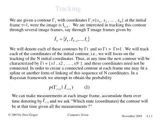
Tracking We are given a contour G1 with coordinates G1={x1 , x2 , … , xN} at the initial frame t=1, were the image is It=1 . We are interested in tracking this contour through several image frames, say through T image frames given by We will denote each of these contours by Gt and so G1 = Gt=1 . We will track each of the coordinates of the initial contour, i.e., we will focus on the tracking of the N initial coordinates. Thus, at any time the new contour will be characterized by Gt = {x1 , x2 , … , xN }, and these coordinates need not be connected. In order to create a connected contour at each frame one may fit a spline or another form of linking of this sequence of N coordinates. In a Bayesian framework we attempt to obtain the probability We can make measurements at each image frame, accumulate them over time denoting by and we ask “Which state (coordinates) the contour will be at that time given all the measurements ?” Computer Vision
Propagating Probability Density An interesting expansion of (1) is given by: Correct or make Measurements Predict Assuming that such probabilities can be obtained, namely than we have a recursive method to estimate Computer Vision
Assumptions Independence assumption on data generation, i.e., the current state completely defines the probability of the measurements/data (often the previous data is also neglected) First order Markov process, i.e., the current state of the system is completely described by the immediate previous state, and possibly the data (often the data is also neglected). This is a normalization constant that can always be computed by normalizing the recurrence equation (2) Computer Vision
Linear Dynamics Examples Random Walk Points moving with constant velocity Points moving with constant acceleration Periodic motion Computer Vision
Random Walk of a Point Drift: New position is the previous one plus noise (sd) Computer Vision
Point moving with constant velocity Computer Vision
Point moving with constant acceleration Computer Vision
Point moving with periodic motion Computer Vision
Tracking one point (dynamic programming like) Equation (2) is written as S S t t-1 t Computer Vision
Kalman Filter (Special Case of a Linear System) Simplify calculation of the probabilities due to good Gaussian properties (applied to ) Reminder: From equation (2) we have 1D case: For one dimension point and Gaussian distributions Kalman observed the recurrence: if then where Computer Vision
Kalman Filter and Gaussian Properties Proof: Assume Then Computer Vision
Kalman Filter …(continuing the proof) Computer Vision
Using Kalman Filter Computer Vision
Kalman Filter (Generalization to N-D) Computer Vision

