Download
1 / 53
530 likes | 544 Vues
A F N I & FMRI Introduction, Concepts, Principles. http://afni.nimh.nih.gov/afni. A F N I = A nalysis of F unctional N euro I mages. Developed to provide an environment for FMRI data analyses And a platform for development of new software

E N D
AFNI &FMRIIntroduction, Concepts, Principles http://afni.nimh.nih.gov/afni
AFNI = Analysis of Functional NeuroImages • Developed to provide an environment for FMRI data analyses • And a platform for development of new software • AFNI refers to both the program of that name and the entire package of external programs and plugins (more than 100) • Important principles in the development of AFNI: • Allow user to stay close to the data and view it in many different ways • Give users the power to assemble pieces in different ways to make customized analyses • “With great power comes great responsibility” — to understand • “Provide mechanism, not policy” • Allow other programmers to add features that can interact with the rest of the package
Principles (and Caveats) We* Live By • Fix significant bugs as soon as possible • But, we define “significant” • Nothing is secret or hidden (AFNI is open source) • But, possibly not very well documented or advertised • Release early and often • All users are beta-testers for life • Help the user (message board; consulting with NIH users) • Until our patience expires • Try to anticipate users’ future needs • What we think you will need may not be what you actually end up needing *
Outline of This Talk • Quick introduction to FMRI physics and physiology • So you have some idea of what is going on in the scanner and what is actually being measured • Brief discussion of FMRI experimental designs • Block, Event-Related, Hybrid Event-Block • But this is not a course in how to design your FMRI experimental paradigm • Outlines of standard FMRI processing pipeline (AFNI-ized) • Keep this in mind for the rest of the class! • Many experiments require tweaking this “standard” collection of steps to fit the design of the paradigm and/or the inferential goals • Overview of basic AFNI concepts • Datasets and file formats; Realtime input; Controller panels; SUMA; Batch programs and Plugins
Quick Intro to MRI and FMRI Physics and Physiology (in pretty small doses) MRI = Cool (and useful) Pictures 2D slices extracted from a 3D (volumetric) image [resolution about 111 mm ; acquisition time about 10 min]
Synopsis of MRI 1) Put subject in big magnetic field (leave him there) 2) Transmit radio waves into subject [about 3 ms] 3) Turn off radio wave transmitter 4) Receive radio waves re-transmitted by subject • Manipulate re-transmission with magnetic fields during this readout interval [10-100 ms] 5) Store measured radio wave data vs. time • Now go back to 2) to get some more data 6) Process raw data to reconstruct images 7) Allow subject to leave scanner (optional) 8) Process images to extract desired features
[Main magnet and some of its lines of force] [Little magnets lining up with external lines of force] B0 = Big Field Produced by Main Magnet • Purpose is to align H protons in H2O (little magnets) • Units of B are Tesla (Earth’s field is about 0.00005 Tesla) • Typical field used in FMRI is 3 Tesla
Subject is magnetized • Small B0 produces • small net • magnetizationM • Thermal energy tries to randomize alignment of proton magnets • Larger B0 produces • larger net • magnetization M, • lined up with B0 • Reality check: 0.0003% of protons • aligned per Tesla • of B0
Precession of Magnetization M • Magnetic field B causes M to rotate (“precess”) about the direction of B at a frequency proportional to the size of B — 42 million times per second (42 MHz), per Tesla of B • 127 MHz at B = 3 Tesla — range of radio frequencies • If M is not parallel to B, then • it precesses clockwise around • the direction of B. • However, “normal” (fully relaxed)situation has M parallel to B, which means there won’t be any • precession • N.B.: part of M parallel to B (Mz) does not precess
B1 = Excitation (Transmitted) RF Field • Left alone, M will align itself with B in about 2–3 s • No precession no detectable signal • So don’t leave it alone: apply (transmit) a magnetic field B1 that fluctuates at the precession frequency (radio frequency=RF) and points perpendicular to B0 • The effect of the tiny B1is to cause M to spiral away • from the direction of the • static B field • B110–4 Tesla • This is called resonance • If B1 frequency is not close to resonance, B1 has no effect Time = 2–4 ms
Readout RF • When excitation RF is turned off, M is left pointed off at some angle to B0 [flip angle] • Precessing part of M [Mxy] is like having a magnet rotating around at very high speed (at RF speed: millions of revs/second) • Will generate an oscillating voltage in a coil of wires placed around the subject — this is magnetic induction • This voltage is the RF signal = the raw data for MRI • At each instant t, can measure one voltage V(t), which is proportional to the sum of all transverse Mxy inside the coil • Must separate signals originating from different regions • By reading out data for 5-60 ms, manipulating B field, being clever … • Then have image of Mxy = map of how much signal from each voxel
Relaxation: Nothing Lasts Forever • In the absence of external B1, M will go back to being aligned with static field B0 = relaxation • Part of M perpendicular to B0 shrinks [Mxy] • This part of M = transverse magnetization • It generates the detectable RF signal • The relaxation of Mxy during readout affects the image • Part of M parallel to B0 grows back [Mz] • This part of M = longitudinal magnetization • Not directly detectable, but is converted into transverse magnetization by external B1 • Therefore, Mz is the ultimate source of the NMR signal, but is not the proximate source of the signal } Time scale for this relaxation is called T2 or T2* = 20-40 ms in brain } Time scale for this relaxation is called T1 = 500-2500 ms
Material Induced Inhomogeneities in B • Adding a nonuniform object (like a person) toB0will make the total magnetic field Bnonuniform • This is due to susceptibility: generation of extra magnetic fields in materials that are immersed in an external field • Diamagnetic materials produce negativeBfields [most tissue] • Paramagnetic materials produce positiveBfields [deoxyhemoglobin] • Size of changes about 10–7B0 = 1–100 Hz change in precession f • Makes the precession frequency nonuniform, which affects the image intensity and quality • For large scale (100+ mm) inhomogeneities, scanner-supplied nonuniform magnetic fields can be adjusted to “even out” the ripples inB— this is called shimming • Nonuniformities inBbigger than voxel size distort whole image • Nonuniformities in Bsmaller than voxel size affect voxel “brightness”
The Concept of Contrast (or Weighting) • Contrast = difference in RF signals — emitted by water protons — between different tissues • Example: gray-white contrast is possible because T1 is different between these two types of tissue
Types of Contrast Used in Brain FMRI • T1 contrast at high spatial resolution • Technique: use very short timing between RF shots (small TR) and use large flip angles • Useful for anatomical reference scans • 5-10 minutes to acquire 256256128 volume • 1 mm resolution easily achievable • finer voxels are possible, but acquisition time increases a lot • T2 (spin-echo) and T2* (gradient-echo) contrast • Useful for functional activation studies • 100 ms per 6464 2D slice 2-3 s to acquire whole brain • 4 mm resolution • better is possible with better gradient system, and/or multiple RF readout coils
What is Functional MRI? • 1991: Discovery that MRI-measurable signal increases a few % locally in the brain subsequent to increases in neuronal activity (Kwong, et al.) Cartoon of MRI signal in an “activated” brain voxel
How FMRI Experiments Are Done • Alternate subject’s neural state between 2 (or more) conditions using sensory stimuli, tasks to perform, ... • Can only measure relative signals, so must look for changes in the signal between the conditions • Acquire MR images repeatedly during this process • Search for voxels whose NMR signal time series (up-and-down) matches the stimulus time series pattern (on-and-off) • Signal changes due to neural activity are small • Need 1000 or so images in time series (each slice) takes an hour or so to get reliable activation maps • Must break image acquisition into shorter “runs” to give the subject and scanner some break time • Other small effects can corrupt the results postprocess the data to reduce these effects & be careful • Lengthy computations for image recon and temporal pattern matching data analysis usually done offline
“Active” voxels Some Sample Data Time Series • 16 slices, 6464 matrix, 68 repetitions (TR=5 s) • Task: phoneme discrimination: 20 s “on”, 20 s “rest” graphs of 9 voxel time series t
One Fast Image Graphs vs. time of 33 voxel region This voxel did not respond Overlay on Anatomy Colored voxels responded to the mental stimulus alternation, whose pattern is shown in the yellow reference curve plotted in the central voxel 68 points in time 5 s apart; 16 slices of 6464 images
Why (and How) Does NMR Signal ChangeWith Neuronal Activity? • There must be something that affects the water molecules and/or the magnetic field inside voxels that are “active” • neural activitychangesblood flow and oxygen usage • blood flow changes which H2O molecules are present and also changes the magnetic field locally • FMRI is thus doubly indirect from physiology of interest (synaptic activity) • also is much slower: 4-6 seconds after neurons • also “smears out” neural activity: cannot resolve 10-100 ms timing of neural sequence of events
Neurophysiological Changes & FMRI • There are 4 changes caused by neural activty that are currently observable using MRI: • Increased Blood Flow • New protons flow into slice from outside • More protons are aligned with B0 • Equivalent to a shorter T1 (as if protons are realigned faster) • NMR signal goes up [mostly in arteries] • Increased Blood Volume (due to increased flow) • Total deoxyhemoglobin increases (as veins expand) • Magnetic field randomness increases [more paramagnetic stuff in blood vessels] • NMR signal goes down [near veins and capillaries]
BUT: “Oversupply” of oxyhemoglobin after activation • Total deoxyhemoglobin decreases • Magnetic field randomness decreases [less paramag stuff] • NMR signal goes up [near veins and capillaries] • This is the important effect for FMRI as currently practiced • Increased capillary perfusion • Most inflowing water molecules exchange to parenchyma at capillaries • i.e., the water that flows into a brain capillary is not the water that flows out! • Can be detected with perfusion-weighted imaging methods • This factoid is also the basis for 15O water-based PET • May someday be important in FMRI, but is hard to do now
Cartoon of Veins inside a Voxel Deoxyhemo-globin is paramagnetic(increases B) Rest of tissue +oxyhemoglobin is diamagnetic (decreases B)
BOLD Contrast • BOLD = Blood Oxygenation Level Dependent • Amount of deoxyhemoglobin in a voxel determines how inhomogeneous that voxel’s magnetic field is at the scale of the blood vessels (and red blood cells) • Increase in oxyhemoglobin in veins after neural activation means magnetic field becomes more uniform inside voxel • So NMR signal goes up (T2 and T2* are larger), since it doesn’t decay as much during data readout interval • So MR image is brighter during “activation” (a little) • Summary: • NMR signal increases 4-6 s after “activation”, due to hemodynamic (blood) response • Increase is same size as noise, so need lots of data
FMRI Experiment Design and Analysis • FMRI experiment design • Event-related, block, hybrid event-block? • How many types of stimuli? How many of each type? Timing (intra- & inter-stim)? • Will experiment show what you are looking for? (Hint: bench tests) • How many subjects do you need? (Hint: the answer does not have 1 digit) • Time series data analysis (individual subjects) • Assembly of images into AFNI datasets; Visual & automated checks for bad data • Registration of time series images • Smoothing & masking of images; Baseline normalization; Censoring bad data • Catenation into one big dataset • Fit statistical model of stimulus timing+hemodynamic response to time series data • Fixed-shape or variable-shape response models • Segregation into differentially active blobs • Thresholding on statistic + clustering and/or Anatomically-defined ROI analysis • Visual examination of maps and fitted time series for validity and meaning • Group analysis (inter-subject) • Spatial normalization to Talairach-Tournoux atlas (or something like it) • Smoothing of fitted parameters • Automatic global smoothing + voxel-wise analysis or ROI averaging • ANOVA to combine and contrast activation magnitudes from the various subjects • Visual examination of results (usually followed by confusion) • Write paper, argue w/ mentor, submit paper, argue w/ referees, publish paper, …
FMRI Experiment Design - 1 • Recall hemodynamic (FMRI) response • peak is 4-6 s after neural activation • width is 4-5 s for very brief (< 1 s) activation • two separate activations less than 12-15 s apart will have their responses overlap and add up (approximately — more on this in a later talk!) • Block design experiments: Extended activation, or multiple closely-spaced activations • Multiple FMRI responses overlap and add up to something more impressive than a single brief blip • But can’t distinguish distinct but closely-spaced activations; example: • Each brief activation is “subject sees a face for 1 s, presses button #1 if male, #2 if female” and faces come in every 2 s for a 20 s block, then 20 s of “rest”, then a new faces block, etc. • What to do about trials where the subject makes a mistake? These are presumably neurally different than correct trials, but there is no way to separate out the activations when the hemodynamics blurs so much in time.
FMRI Experiment Design - 2 • Event-related designs: • Separate activations in time so can model the FMRI response from each separately, as needed (e.g., in the case of subject mistakes) • Need to make inter-stimulus intervals vary (“jitter”) if there is any potential time overlap in their FMRI response curves; e.g., if the events are closer than 12-15 s in time • Otherwise, the tail of event #x always overlaps the head of event #x+1 in the same way, and as a result the amplitude of the response in the tail of #x can’t be told from the response in the head of #x+1 • Important note! • You cannot treat every single event as a distinct entity whose response amplitude is to be calculated separately! • You must still group events into classes, and assume that all events in the same class evoke the same response. • There is just too much noise in FMRI to be able to get an accurate activation map from a single event!
FMRI Experiment Design - 3 • Hybrid Block/Event-related designs: • The long “blocks” are situations where you set up some continuing condition for the subject • Within this condition, multiple distinct events are given • Example: • Event stimulus is a picture of a face • Block condition is instruction on what the subject is to do when he sees the face: • Condition A: press button #1 for male, #2 for female • Condition B: press button #1 if face is angry, #2 if face is happy • Event stimuli in the two conditions may be identical, or at least fungible • It is the instructional+attentional modulation between the two conditions that is the goal of such a study • Perhaps you have two groups of subjects (patients and controls) which respond differently in bench tests • You want to find some neural substrates for these differences
3D Individual Subject Analysis to3d OR can do at scanner Assemble images into AFNI-formatted datasets Check images for quality (visual & automatic) afni + 3dToutcount 3dvolreg OR 3dWarpDrive Register (realign) images Smooth images spatially 3dmerge (optional) Mask out non-brain parts of images 3dAutomask + 3dcalc (optional) 3dTstat + 3dcalc (optional: could be done post-fit) Normalize time series baseline to 100 (for %-izing) • Fit stimulus timing + hemodynamic model to time series • catenates imaging runs, removes residual movement effects, computes response sizes & inter-stim contrasts 3dDeconvolve Alphasim + 3dmerge OR Extraction from ROIs Segregate into differentially “activated” blobs afni AND your personal brain Look at results, and think … to group analysis (next page)
Group Analysis: in 3D or on folded 2D cortex models Datasets of results from individual subject analyses Construct cortical surface models Normalize datasets to Talairach “space” Project 3D /results to cortical surface models OR Smooth fitted response amplitudes Average fitted response amplitudes over ROIs OR Use ANOVA to combine + contrast results View and understand results; Write paper; Start all over
Fundamental AFNI Concepts • Basic unit of data in AFNI is the dataset • A collection of 1 or more 3D arrays of numbers • Each entry in the array is in a particular spatial location in a 3D grid (a voxel= 3D pixel) • Image datasets: each array holds a collection of slices from the scanner • Each number is the signal intensity for that particular voxel • Derived datasets: each number is computed from other dataset(s) • e.g., each voxel value is a t-statistic reporting “activation” significance from an FMRI time series dataset, for that voxel • Each 3D array in a dataset is called a sub-brick • There is one number in each voxel in each sub-brick } 3x3x3 Dataset With 4 Sub-bricks
and I mean this Dataset Contents: Numbers • Different types of numbers can be stored in datasets • 8 bit bytes (e.g., from grayscale photos) • 16 bit short integers (e.g., from MRI scanners) • Each sub-brick may also have a floating point scale factor attached, so that “true” value in each voxel is actually (value in dataset file) • 32 bit floats (e.g., calculated values; lets you avoid the ) • 24 bit RGB color triples (e.g., JPEGs from your digital camera!) • 64 bit complex numbers (e.g., for the physicists in the room) • Different sub-bricks are allowed to have different numeric types • But this is not recommended • Will occur if you “catenate” two dissimilar datasets together (e.g., using 3dTcat or 3dbucket commands) • Programs will display a warning to the screen if you try this
Dataset Contents: Header • Besides the voxel numerical values, a dataset also contains auxiliary information, including (some of which is optional): • xyz dimensions of each voxel (in mm) • Orientation of dataset axes; for example, x-axis=R-L, y-axis=A-P, z-axis=I-S axial slices (we call this orientation “RAI”) • Location of dataset in scanner coordinates • Needed to overlay one dataset onto another • Very important to get right in FMRI, since we deal with many datasets • Time between sub-bricks, for 3D+time datasets • Such datasets are the basic unit of FMRI data (one per imaging run) • Statistical parameters associated with each sub-brick • e.g., a t-statistic sub-brick has degrees-of-freedom parameter stored • e.g., an F-statistic sub-brick has 2 DOF parameters stored
AFNI Dataset Files - I • AFNI formatted datasets are stored in 2 files • The .HEAD file holds all the auxiliary information • The .BRIK file holds all the numbers in all the sub-bricks • Datasets can be in one of 3 coordinate systems (AKA views) • Original data or +orig view: from the scanner • AC-PC aligned or +acpc view: • Dataset rotated/shifted so that the anterior commissure and posterior commissure are horizontal (y-axis), the AC is at (x,y,z)=(0,0,0), and the hemispheric fissure is vertical (z-axis) • Talairach or +tlrc view: • Dataset has also been rescaled to conform to the Talairach-Tournoux atlas dimensions (R-L=136 mm; A-P=172 mm; I-S=116 mm) • AKA Talairach or Stererotaxic coordinates • Not quite the same as MNI coordinates, but very close
AFNI Dataset Files - II • AFNI dataset filenames consist of 3 parts • The user-selected prefix (almost anything) • The view (one of +orig, +acpc, or +tlrc) • The suffix (one of .HEAD or .BRIK) • Example: BillGates+tlrc.HEAD and BillGates+tlrc.BRIK • When creating a dataset with an AFNI program, you supply the prefix; the program supplies the rest • AFNI programs can read datasets stored in several formats • ANALYZE (.hdr/.img file pairs); i.e., from SPM, FSL • MINC-1 (.mnc); i.e., from mnitools • CTF (.mri, .svl) MEG analysis volumes • ASCII text (.1D) — numbers arranged into columns • Have conversion programs to write out MINC-1, ANALYZE, ASCII, and NIfTI-1.1 files from AFNI datasets, if desired
NIfTI Dataset Files • NIfTI-1.1 (.niior.nii.gz) is a new standard format that AFNI, SPM, FSL, BrainVoyager, et al., have agreed upon • Adaptation and extension of the old ANALYZE 7.5 format • Goal: easier interoperability of tools from various packages • All data is stored in 1 file (cf. http://nifti.nimh.nih.gov/) • 348 byte header (extensions allowed; AFNI uses this feature) • Followed by the image numerical values • Allows 1D-5D datasets of diverse numerical types • .nii.gz suffix means file is compressed (with gzip) • AFNI now reads and writes NIfTI-1.1 formatted datasets • To write: when you give the prefix for the output filename, end it in “.nii” or “.nii.gz”, and all AFNI programs will automatically write NIfTI-1.1 format instead of .HEAD/.BRIK • To read: just give the full filename ending in “.nii” or “.nii.gz”
Dataset Directories • Datasets are stored in directories, also called sessions • All the datasets in the same session, in the same view, are presumed to be aligned in xyz-coordinates • Voxels with same value of (x,y,z) correspond to same brain location • Can overlay (in color) any one dataset on top of any other one dataset (in grayscale) from same session • Even if voxel sizes and orientations differ • Typical AFNI contents of a session directory are all data derived from a single scanning session for one subject • Anatomical reference (T1-weighted SPGR or MP-RAGE volume) • 10-20 3D+time datasets from FMRI EPI functional runs • Statistical datasets computed from 3D+time datasets, showing activation (you hope and pray) • Datasets transformed from +orig to +tlrc coordinates, for comparison and conglomeration with datasets from other subjects
Getting and Installing AFNI • AFNI runs on Unix systems: Linux, Sun, SGI, Mac OS X • Can run under Windows with Cygwin Unix emulator • This option is really just for trying it out — not for production use • If you are at the NIH: SSCC can install AFNI and update it on your system(s) • You must give us an account with ssh access • You can download precompiled binaries from our Website • http://afni.nimh.nih.gov/afni • Also: documentation, message board, humor, data, … • You can download source code and compile it • AFNI is updated fairly frequently, so it is important to update occasionally • We won’t help you with old versions!
AFNI at the NIH Scanners • AFNI can take images in “realtime” from an external program and assemble them into 3D+time datasets slice-by-slice • Recently (July 2005), Jerzy Bodurka (FMRIF) has set up the GE Excite-based scanners (3T-1, 1.5 T, NMRF 3 T, and 7 T) to start AFNI automagically when scanning, and send reconstructed images over as soon as they are available: • For immediate display (images and graphs of time series) • Plus graphs of estimate subject head movement • Goal is to let you see data as it is acquired, so that if there are any big problems, you can fix them right away • Sample problem: someone typed in the imaging field-of-view (FOV) size wrong (240 cm instead of 24 cm), and got garbage data, but only realized this too late (after subject had left the scanner and gone home) — D’oh!
A Quick Overview of AFNI • Starting AFNI from the Unix command line • afni reads datasets from the current directory • afni dir1 dir2 … reads datasets from directories listed • afni -R reads datasets from current directory and from all directories below it • AFNI also reads a file named .afnirc from your home directory • Used to change many of the defaults • Window layout and image/graph viewing setup; popup hints; whether to compress .BRIK files when writing • cf. file README.environment in the AFNI documentation • Also can read file .afni.startup_script to restore the window layout from a previous run • Created from Define Datamode->Misc->Save Layout menu • cf. file README.driver for what can be done with AFNI scripts
AFNI controller window at startup Titlebar shows current datasets Switch to different coordinate system Coordinates of current focus point Markers control transformation to +acpc and +tlrc coordinates Control crosshairs appearance Time index Controls color functional overlay Open images and graphs of datasets Miscellaneous menus Open new AFNI controller Switch between directories, underlay (anatomical) datasets, and overlay (functional) datasets Help Button Controls display of overlaid surfaces Close this controller
Disp and Mont control panels AFNI Image Viewer
AFNI Time Series Graph Viewer Data (black) and Reference waveforms (red) Menus for controlling graph displays
Define Overlay: Colorizing Panel (etc.) Color map Hidden popup menu here Choose which dataset makes the underlay image Choose which sub-brick from Underlay dataset to display (usu. Anat - has only 1 sub-brick) Threshold slider Choose which sub-brick of functional dataset makes the color Choose which sub-brick of functional dataset is the Threshold p-value of current threshold Shows ranges of data in Underlay and Overlay dataset Choose range of threshold slider, in powers of 10 Shows automatic range for color scaling Rotates color map Positive-only or both signs of function? Number of panes in color map Shows voxel values at focus Lets you choose range for color scaling
Pick new underlay dataset Name of underlay dataset Sub-brick to display Volume Rendering: an AFNI plugin Open color overlay controls Range of values in underlay Range of values to render Change mapping from values in dataset to brightness in image Histogram of values in underlay dataset Mapping from values to opacity Maximum voxel opacity Menu to control scripting (control rendering from a file) Cutout parts of 3D volume Compute many images in a row Render new image immediately when a control is changed Show 2D crosshairs Control viewing angles Accumulate a history of rendered images (can later save to an animation) Reload values from the dataset Force a new image to be rendered Detailed instructions Close all rendering windows
Staying Close to Your Data! “ShowThru” rendering of functional activation: animation created with Automate and Save:aGif controls
Other Parts of AFNI • Batch mode programs • Are run by typing commands directly to computer, or by putting commands into a text file (script) and later executing them • Good points about batch mode • Can process new datasets exactly the same as old ones • Can link together a sequence of programs to make a customized analysis (a personalized pipeline) • Some analyses take a long time • Bad points about batch mode • Learning curve is “all at once” rather than gradual • If you are, like, under age 35, you may not know how to type commands into a computer • At least we don’t make you use punched cards (yet)
AFNI Batch Programs • Many important capabilities in AFNI are onlyavailable in batch programs • A few examples (of more than 100, from trivial to complex) • 3dDeconvolve= multiple linear regression on 3D+time datasets, to fit each voxel’s time series to an activation model and then test these fits for significance • 3dvolreg = 3D+time dataset registration, to correct for small subject head movements, and for inter-day head positioning • 3dANOVA = 1-, 2-, 3-, and 4- way ANOVA layouts, for combining & contrasting datasets in Talairach space • 3dcalc = general purpose voxel-wise calculator • 3dclust = find clusters of activated voxels • 3dresample = re-orient and/or re-size dataset voxel grid • 3dSkullStrip = remove “skull” from anatomical dataset
AFNI Plugins • A plugin is an extension to AFNI that attaches itself to the interactive AFNI GUI • Not the same as a batch program • Offers a relatively easy way to add certain types of interactive functionality to AFNI • A few examples: • Draw Dataset = ROI drawing (draws numbers into voxels) • Render [new] = Volume renderer • Dataset#N = Lets you plot multiple 3D+time datasets as overlays in an AFNI graph viewer (e.g., fitted model over data) • Histogram = Plots a histogram of a dataset or piece of one • Edit Tagset = Lets you attach labeled “tag points” to a dataset (e.g., as anatomical reference markers)
SUMA, et alii • SUMA is the AFNI surface mapper • For displaying surface models of the cortex • Surface models come from FreeSurfer (MGH) or SureFit/Caret (Wash U) or BrainVoyager • Can display functional activations mapped from 3D volumes to the cortical surface • Can draw ROIs directly on the cortical surface • vs. AFNI: ROIs are drawn into the volume • SUMA is a separate program from AFNI, but can “talk” to AFNI so that volume and surface viewing are linked • Click in AFNI or SUMA to change focus point, and the other program jumps to that location at the same time • Functional overlay in AFNI can be sent to SUMA for simultaneous display • And much more — stayed tuned for the SUMA talks to come!