Lecture 7 - Meshing Applied Computational Fluid Dynamics
Lecture 7 - Meshing Applied Computational Fluid Dynamics. Instructor: André Bakker. © André Bakker (2002-2005) © Fluent Inc. (2002). Outline. Why is a grid needed? Element types. Grid types. Grid design guidelines. Geometry. Solution adaption. Grid import. Why is a grid needed?.

Lecture 7 - Meshing Applied Computational Fluid Dynamics
E N D
Presentation Transcript
Lecture 7 - MeshingApplied Computational Fluid Dynamics Instructor: André Bakker © André Bakker (2002-2005) © Fluent Inc. (2002)
Outline • Why is a grid needed? • Element types. • Grid types. • Grid design guidelines. • Geometry. • Solution adaption. • Grid import.
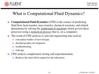
Why is a grid needed? • The grid: • Designates the cells or elements on which the flow is solved. • Is a discrete representation of the geometry of the problem. • Has cells grouped into boundary zones where b.c.’s are applied. • The grid has a significant impact on: • Rate of convergence (or even lack of convergence). • Solution accuracy. • CPU time required. • Importance of mesh quality for good solutions. • Grid density. • Adjacent cell length/volume ratios. • Skewness. • Tet vs. hex. • Boundary layer mesh. • Mesh refinement through adaption.
Geometry • The starting point for all problems is a “geometry.” • The geometry describes the shape of the problem to be analyzed. • Can consist of volumes, faces (surfaces), edges (curves) and vertices (points). Geometry can be very simple... … or more complex geometry for a “cube”
Geometry creation • Geometries can be created top-down or bottom-up. • Top-down refers to an approach where the computational domain is created by performing logical operations on primitive shapes such as cylinders, bricks, and spheres. • Bottom-up refers to an approach where one first creates vertices (points), connects those to form edges (lines), connects the edges to create faces, and combines the faces to create volumes. • Geometries can be created using the same pre-processor software that is used to create the grid, or created using other programs (e.g. CAD, graphics).
Typical cell shapes • Many different cell/element and grid types are available. Choice depends on the problem and the solver capabilities. • Cell or element types: • 2D: • 3D: 2D prism (quadrilateral or “quad”) triangle (“tri”) prism with quadrilateral base (hexahedron or “hex”) tetrahedron(“tet”) prism with triangular base (wedge) pyramid arbitrary polyhedron
Cell = control volume into which domain is broken up. Node = grid point. Cell center = center of a cell. Edge = boundary of a face. Face = boundary of a cell. Zone = grouping of nodes, faces, and cells: Wall boundary zone. Fluid cell zone. Domain = group of node, face and cell zones. Terminology node cell center face cell 2D computational grid node edge cell face 3D computational grid
Grid types: structured grid • Single-block, structured grid. • i,j,k indexing to locate neighboring cells. • Grid lines must pass all through domain. • Obviously can’t be used for very complicated geometries.
+ + + + Face meshing: structured grids • Different types of hexahedral grids. • Single-block. • The mesh has to be represented in a single block. • Connectivity information (identifying cell neighbors) for entire mesh is accessed by three index variables: i, j, k. Single-block geometry Logical representation. • Single-block meshes may include 180 degree corners.
Grid types: multiblock • Multi-block, structured grid. • Uses i,j,k indexing within each mesh block. • The grid can be made up of (somewhat) arbitrarily-connected blocks. • More flexible than single block, but still limited. Source: www.cfdreview.com
Face meshing: multiblock • Different types of hexahedral grids. • Multi-block. • The mesh can be represented in multiple blocks. Multi-block geometry Logical representation. • This structure gives full control of the mesh grading, using edge meshing, with high-quality elements. • Manual creation of multi-block structures is usually more time-consuming compared to unstructured meshes.
Grid types: unstructured • Unstructured grid. • The cells are arranged in an arbitrary fashion. • No i,j,k grid index, no constraints on cell layout. • There is some memory and CPU overhead for unstructured referencing. Unstructured mesh on a dinosaur
Unstructured Grid Face meshing: unstructured grids • Different types of hexahedral grids. • Unstructured. • The mesh has no logical representation.
Face meshing: quad examples • Quad: Map. • Quad: Submap. • Quad: Tri-Primitive. • Quad: Pave and Tri-Pave.
Grid types: hybrid • Hybrid grid. • Use the most appropriate cell type in any combination. • Triangles and quadrilaterals in 2D. • Tetrahedra, prisms and pyramids in 3D. • Can be non-conformal: grids lines don’t need to match at block boundaries. prism layer efficiently resolves boundary layer tetrahedral volume mesh is generated automatically triangular surface mesh on car body is quick and easy to create non-conformal interface
Start from 3D boundary mesh containing only triangular faces. Generate mesh consisting of tetrahedra. Tetrahedral mesh Complex Geometries Surface mesh for a grid containing only tetrahedra
Flow alignment well defined in specific regions. Start from 3D boundary and volume mesh: Triangular and quadrilateral faces. Hexahedral cells. Generate zonal hybrid mesh, using: Tetrahedra. Existing hexahedra. Transition elements: pyramids. Zonal hybrid mesh Surface mesh for a grid containing hexahedra, pyramids, and tetrahedra (and prisms)
Parametric study of complex geometries. Nonconformal capability allows you to replace portion of mesh being changed. Start from 3D boundary mesh or volume mesh. Add or replace certain parts of mesh. Remesh volume if necessary. Nonconformal mesh Nonconformal mesh for a valve port nonconformal interface
Mesh naming conventions - topology • Structured mesh: the mesh follows a structured i,j,k convention. • Unstructured mesh: no regularity to the mesh. • Multiblock: the mesh consists of multiple blocks, each of which can be either structured or unstructured.
Mesh naming conventions – cell type • Tri mesh: mesh consisting entirely of triangular elements. • Quad mesh: consists entirely of quadrilateral elements. • Hex mesh: consists entirely of hexahedral elements. • Tet mesh: mesh with only tetrahedral elements. • Hybrid mesh: mesh with one of the following: • Triangles and quadrilaterals in 2D. • Any combination of tetrahedra, prisms, pyramids in 3D. • Boundary layer mesh: prizms at walls and tetrahedra everywhere else. • Hexcore: hexahedra in center and other cell types at walls. • Polyhedral mesh: consists of arbitrary polyhedra. • Nonconformal mesh: mesh in which grid nodes do not match up along an interface.
1. Create, read (or import) boundary mesh(es). 2. Check quality of boundary mesh. 3. Improve and repair boundary mesh. 4. Generate volume mesh. 5. Perform further refinement if required. 6. Inspect quality of volume mesh. 7. Remove sliver and degenerate cells. 8. Save volume mesh. Mesh generation process Surface mesh for a grid containing only tetrahedra
Two phases: Initial mesh generation: Triangulate boundary mesh. Refinement on initial mesh: Insert new nodes. Tri/tet grid generation process Initial mesh Cell zone refinement Boundary refinement
Mesh quality • For the same cell count, hexahedral meshes will give more accurate solutions, especially if the grid lines are aligned with the flow. • The mesh density should be high enough to capture all relevant flow features. • The mesh adjacent to the wall should be fine enough to resolve the boundary layer flow. In boundary layers, quad, hex, and prism/wedge cells are preferred over tri’s, tets, or pyramids. • Three measures of quality: • Skewness. • Smoothness (change in size). • Aspect ratio.
Two methods for determining skewness: 1. Based on the equilateral volume: Skewness = Applies only to triangles and tetrahedra. Default method for tris and tets. 2. Based on the deviation from a normalized equilateral angle: Skewness (for a quad) = Applies to all cell and face shapes. Always used for prisms and pyramids. optimal (equilateral) cell circumcircle actual cell Mesh quality: skewness
max 0 1 bestworst min Equiangle skewness • Common measure of quality is based on equiangle skew. • Definition of equiangle skew: where: • max = largest angle in face or cell. • min = smallest angle in face or cell. • e = angle for equiangular face or cell. • e.g., 60 for triangle, 90 for square. • Range of skewness:
smooth change large jump in in cell size cell size aspect ratio = 1 high-aspect-ratio quad aspect ratio = 1 high-aspect-ratio triangle Mesh quality: smoothness and aspect ratio • Change in size should be gradual (smooth). • Aspect ratio is ratio of longest edge length to shortest edge length. Equal to 1 (ideal) for an equilateral triangle or a square.
Striving for quality • A poor quality grid will cause inaccurate solutions and/or slow convergence. • Minimize equiangle skew: • Hex and quad cells: skewness should not exceed 0.85. • Tri’s: skewness should not exceed 0.85. • Tets: skewness should not exceed 0.9. • Minimize local variations in cell size: • E.g. adjacent cells should not have ‘size ratio’ greater than 20%. • If such violations exist: delete mesh, perform necessary decomposition and/or pre-mesh edges and faces, and remesh.
flow inadequate better Grid design guidelines: resolution • Pertinent flow features should be adequately resolved. • Cell aspect ratio (width/height) should be near one where flow is multi-dimensional. • Quad/hex cells can be stretched where flow is fully-developed and essentially one-dimensional. Flow Direction OK!
Grid design guidelines: smoothness • Change in cell/element size should be gradual (smooth). • Ideally, the maximum change in grid spacing should be <20%: smooth change in cell size sudden change in cell size — AVOID! • • • Dxi Dxi+1
Grid design guidelines: total cell count • More cells can give higher accuracy. The downside is increased memory and CPU time. • To keep cell count down: • Use a non-uniform grid to cluster cells only where they are needed. • Use solution adaption to further refine only selected areas. • Cell counts of the order: • 1E4 are relatively small problems. • 1E5 are intermediate size problems. • 1E6 are large. Such problems can be efficiently run using multiple CPUs, but mesh generation and post-processing may become slow. • 1E7 are huge and should be avoided if possible. However, they are common in aerospace and automotive applications. • 1E8 and more are department of defense style applications.
Solution adaption • How do you ensure adequate grid resolution, when you don’t necessarily know the flow features? Solution-based grid adaption! • The grid can be refined or coarsened by the solver based on the developing flow: • Solution values. • Gradients. • Along a boundary. • Inside a certain region.
Grid adaption • Grid adaption adds more cells where needed to resolve the flow field. • Fluent adapts on cells listed in register. Registers can be defined based on: • Gradients of flow or user-defined variables. • Isovalues of flow or user-defined variables. • All cells on a boundary. • All cells in a region. • Cell volumes or volume changes. • y+ in cells adjacent to walls. • To assist adaption process, you can: • Combine adaption registers. • Draw contours of adaption function. • Display cells marked for adaption. • Limit adaption based on cell size and number of cells.
2D planar shell - final grid 2D planar shell - contours of pressure final grid Adaption example: final grid and solution
Main sources of errors • Mesh too coarse. • High skewness. • Large jumps in volume between adjacent cells. • Large aspect ratios. • Interpolation errors at non-conformal interfaces. • Inappropriate boundary layer mesh.
Summary • Design and construction of a quality grid is crucial to the success of the CFD analysis. • Appropriate choice of grid type depends on: • Geometric complexity. • Flow field. • Cell and element types supported by solver. • Hybrid meshing offers the greatest flexibility. • Take advantage of solution adaption.