Download
1 / 31
310 likes | 673 Vues
Performance analysis of fault detection systems based on analytical redundancy. Timothy J. Wheeler Berkeley Center for Control & Identification Department of Mechanical Engineering University of California, Berkeley. Overview. Introduction Reliability through physical redundancy

E N D
Performance analysis of fault detection systems based on analytical redundancy Timothy J. Wheeler Berkeley Center for Control & IdentificationDepartment of Mechanical EngineeringUniversity of California, Berkeley
Overview • Introduction • Reliability through physical redundancy • Quantifying performance of fault detection schemes • Simple example • Physically redundant configuration • Analytically redundant configuration • Application: air data probe • Performance analysis (requires linearization) • Verification with Monte Carlo estimates • Finding “worstcase” flight path • Future Work
Reliability of avionics systems • FAA certification of safety critical systems is a rigorous process • Failure Modes and Effects Analysis (FMEA) • Fly-by-wire control: < 10-9 catastrophic failures per flight hour • Reliability achieved through physical redundancy • Certification based on hardware failure rates and fault trees • Example: Boeing 777 • 14 spoilers, 2 outboard ailerons, 2 flaperons, 2 elevatorsEach driven by multiple independent actuators • 3 primary flight computers (different processors, compilers) • Increases system power, cost, weight (not suitable for UAVs) • Can analytically redundant systems be this reliable?
Air data probes Used on nearly all aircraft Most air data probes manufactured by Goodrich • Basic Operation • Pitot tube measures total pressure • Static port measures static pressure • Pressures used to compute indicated airspeed and altitude • Failure of these probes has resulted in a number of accidents • 1974: Northwest Flight 6231, Boeing 727, iced pitot tubes • 1996: Birgenair Flight 301, Boeing 757, blocked pitot tube (insects)* • 1996: AeroPeru Flight 603, Boeing 757, tape over static port • 2009: Air France Flight 447, Airbus A330, pitot tube malfunction* • Reliability currently achieved through physical redundancy *suspected
Quantifying performance of fault detection • Breakdown performance into four scenarios • Confusion matrix • Array of probabilities of these events • Probabilities sum to 1 • Only “True Negative” indicates healthy system • Physically redundant case is an extreme example(False Positive and False Negative are negligible)
Simple abstract example • Physically and analytically redundant system • Both systems have two sensors • Each sensorcorrupted by noise & random bias fault • Physical redundancy • Two independent copies of the same sensor measure h • Analytical redundancy • Two different sensors measure other quantities u and v • Analytical relationships used to derive h in two different ways • Fault detection methodology • Subtract hmeasurements to get the residual: r = h1- h2 • Signal “fault” when |rk| > ε, “no fault” when |rk| ≤ ε • In both cases, the performance can be computed directly
Physically redundant system Sensor 1 • Two measurements ofthe same quantity • Sensor noise sequences • White, Gaussian, IID: n1k ~ N(0, σ2), n2k ~ N(0, σ2) • Sensor faults modeled as biases • Magnitude of bias: b • Fault times T1, T2 are geometric random variables Ti ~ Geo(q) • Fault signals: • Sensor faults are independent of sensor noises Sensor 2 Markov Chain 1-q q 0 1 1
Physically redundant system • Computing the residual • Mean: • Variance: • Factorize joint density as • Use this to compute the entries of the confusion matrix Sensor 1 Sensor 2 Gaussian Geometric Easy to evaluate
Analytically redundant system Sensor 1 • Analytical relationships • G is a constant matrix • White, Gaussian, IID noises: • Different std. dev. σ1 and σ2 (same “units” as u and v, respectively) • Fault signals of the same form, but • Fault times have different parameters • Different bias magnitudes b1 and b2 (same “units” as u and v, resp.) • “Integrator” initial condition: Sensor 2
Analytically redundant system • Computing the residual • Again, use factorization Accumulation of noises & biases Affine function of all past noises G can be time-varying Gaussian Geometric Easy to evaluate
Quantifying performance • Confusion matrix (at time k) in terms of conditional densities Gaussian Geometric Gaussian Geometric Gaussian Geometric Gaussian Geometric
Numerical results • Procedure • Fix a time window (k = 1, 2, …, N) • Choose system parameters • Fix values for physically redundant system • Fix a matrix G • Choose parameters for analytically redundant systemto “match” (same variance in h) • Compare confusion matrix entries • Improve the sensors in the analytically redundant case • In this case, smaller noise variances • Compare confusion matrix entries again
Numerical results – comparable sensors 1 TN (A) FP (A) 0.8 TN (P) FP (P) 0.6 Probability 0.4 0.2 0 0 500 1000 1500 2000 0.35 TP (A) 0.3 FN (A) TP (P) 0.25 FN (P) 0.2 Probability 0.15 0.1 0.05 0 0 500 1000 1500 2000 Time step, k • Physical • Analytical
Numerical results – improved sensors 1 TN (A+) FP (A+) 0.8 TN (P) FP (P) 0.6 Probability 0.4 0.2 0 0 500 1000 1500 2000 0.35 TP (A+) 0.3 FN (A+) TP (P) 0.25 FN (P) 0.2 Probability 0.15 0.1 0.05 0 0 500 1000 1500 2000 Time step, k • Physical • Analytical Less noise
Application: Air data probe • Sensor description • Measures total and static pressures • Nonlinear equations to produce analytically redundant altitude measurements • Analysis • Simplifications • Linearize sensor equations • Yields time-varying version of previous analytically redundant system • Compute residual for simplified system • Compute confusion matrix entries • Find worstcase (parameterized) flight path
Air data probe • Nonlinear sensor equations • Constants k1, k2, k3, k4, and p0 model troposphere (up to 36,000 ft) • Sensor noise processes • White, Gaussian, IID: • {Vk} and {hk} are non-Gaussian, correlated random processes total dynamicpressure indicated airspeed altitude static pressure
Air data probe – fault model • Sensor faults modeled as bias in pressure • Magnitude of biases: b1, b2 • Fault times: T1, T2 are geometric random variables Ti ~ Geo(qi) • Fault signals: • Sensor faults are independent of sensor noises Markov Chain 1-q q 0 1 1
Air data probe – analytical redundancy • Augment system with flight path angle measurement γ • For now, assume γ known • Use V and γ to compute climb rate • “Integrator” initial condition • Monitor residual rk to detect faults flight path angle Only holds for true airspeed Must include temperature or restrict to low altitude Could also initializeon the ground (ĥ0=hg)
Air data probe – linearization 4 x 10 500 3 V(kts) h (ft) 0 0 0 6.8 4 15 p (psi) p - p (psi) t s s • Sensor equations are mildly nonlinear • First-order Taylor series expansion • For each k, define matrix • Sequence {Gk} only depends on flight path • Altitude only depends on ps, so Gk,22 = 0 for all k
Air data probe – residual • Computing the residual • Same as analytically redundant system, but time-varying • Statistics of residual • Again, use factorization Accumulation of noises & biases Drifting mean Increasing variance Gaussian Geometric Easy to evaluate
Air data probe – numerical results o Calculated • MC estimate
Air data probe – numerical results o Calculated • MC estimate
Air data probe – worstcase flight path • Procedure • Fix a time step k • Choose an objective function • Expressed in terms of Pr( True Neg. ), Pr( False Pos. ), etc. • Parameterize flight path {Vk}, {hk} and {γk} • Examples: level flight, steady climb/decent, altitude profile • Find parameters that maximize the objective
Worstcase flight path – objective • Define events • Possible objectives: Find flight path that… • Maximizes probability of error at time step k • Minimizes probability of True Negative at time step k • EF is independent of noises and flight path, so “No fault yet” “Some fault occurred” Competing terms
Worstcase flight path – results • Level flight • Constant airspeed, constant altitude (γ= 0) • Steady climb/descent • Constant airspeed, constant flight path angle Lower bound (fmincon)
Worstcase flight path – results • Polynomial altitude profile • Constant velocity • Altitude parameterized by Chebyshev polynomials Lower bound (fmincon)
Extension to larger sensor systems B1 A1 C1 MVS,etc. MVS,etc. MVS,etc. C2 B2 A2 A3 B3 C3 A B • Analytical Redundancy • Only 3sensors • Possible3-fold comparison • Map Gmay increase uncertainty • Physical Redundancy • m-plex requires 3msensors • Minimal uncertainty in residual C
Future work • More sophisticated hypothesis testing • Find “optimal” threshold ε • Optimal in what sense? • Bayesian approach • Assign a risk (cost) to each event (False Neg., False Pos., etc.) • Choose “decision function” to minimize risk • Likelihood ratio test • H0,k no fault yet at time k • H1,k some fault before time k • Set threshold on likelihood ratio • Extend to arbitrary linear dynamics • Anticipate residual will still be affine in noises and faults • Extend to nonlinear dynamics
Extension to nonlinear systems P • Linear H∞ filter design (Freeman, Seiler, Balas) • Linearized dynamics, linear filter • Design process • Get filter for many trim conditions • Piece together with gain scheduling, LPV • Can nonlinear filter achieve similar or better performance? • One design for entire flight envelope GTM plant sensors
Nonlinear filtering • Many popular techniques • Unscented Kalman filters • Particle filters • Multiple-model methods • Hybrid system with different modes (nominal, fault 1, fault 2, etc.) • Estimate state of system and mode simultaneously • Analysis of performance • Monte Carlo simulations
Acknowledgements • Advisor • Prof. Andrew PackardDepartment of Mechanical EngineeringUniversity of California Berkeley • Hosts & Collaborators • Prof. Gary Balas • Dr. Peter Seiler • Funding • NASA Hyper X Project (Grant NNX07AC40A)