Data Organization - B-trees
Data Organization - B-trees. General Overview. Relational model - SQL Formal & commercial query languages Functional Dependencies Normalization Physical Design Indexing Query evaluation Query optimization …. Application Oriented. Systems Oriented. Storage Media: Types.

Data Organization - B-trees
E N D
Presentation Transcript
General Overview • Relational model - SQL • Formal & commercial query languages • Functional Dependencies • Normalization • Physical Design • Indexing • Query evaluation • Query optimization • …. Application Oriented Systems Oriented
Storage Media: Types • Cache – fastest and most costly form of storage; volatile; managed by the computer system hardware. • Main memory: • fast access (10s to 100s of nanoseconds; 1 nanosecond = 10–9 seconds) • generally too small (or too expensive) to store the entire database (but for some applications, this is changing) • Volatile — contents of main memory are usually lost if a power failure or system crash occurs. • But… CPU operates only on data in main memory
Storage Media: Types (cont.) • Disk • Primary medium for the long-term storage of data; typically stores entire database. • random-access – possible to read data on disk in any order, unlike magnetic tape • Non-volatile: data survive a power failure or a system crash, disk failure less likely than them • Flash Memory • no seeks • Cheap reads, expensive writes • experimental use for DB’s • NVM
Memory Hierarchy cache Main memory Volatile Non-Volatile Lower price Flash Higher speed disk Optical storage Traveling the hierarchy: 1. speed ( higher=faster) 2. cost (lower=cheaper) 3. volatility (between MM and Disk) 4. Data transfer (Main memory the “hub”) 5. Storage classes (P=primary, S=secondary, T=tertiary)
Read-write head • Positioned very close to the platter surface (almost touching it) • Surface of platter divided into circular tracks • Each track is divided into sectors. • A sector is the smallest unit of data that can be read or written. • To read/write a sector • disk arm swings to position head on right track • platter spins continually; data is read/written as sector passes under head • Block: a sequence of sectors • Cylinder iconsists of ith track of all the platters Top view
Performance Measures of Disks Measuring Disk Speed • Access time – consists of: • Seek time – time it takes to reposition the arm over the correct track. • (Rotational) latency time – time it takes for the sector to be accessed to appear under the head. • Data-transfer rate– the rate at which data can be retrieved from or stored to the disk. Analogy to taking a bus: 1. Seek time: time to get to bus stop 2. Latency time; time spent waiting at bus stop 3. Data transfer time: time spent riding the bus
Random vs sequential I / O • Ex: 1 KB Block • Random I/O: 20 ms. • Sequential I/O: 1 ms. Rule of Random I/O: ExpensiveThumb Sequential I/O: Much less ~10-20 times
Data organization and retrieval File organization can improve data retrieval time 100 blocks 200 recs/block Query returns 150 records SELECT * FROM depositors WHERE bname=“Downtown” Ordered File Heap Brighton A-217 Downtown A-101 Downtown A-110 ...... Mianus A-215 Perry A-218 Downtown A-101 .... OR Searching a heap: must search all blocks (100 blocks) Searching an ordered file: 1. Binary search for the 1st tuple in answer : log2 100 = 7 block accesses 2. scan blocks with answer: no more than 2 Total <= 9 block accesses
Data organization and retrieval But... file can only be ordered on one search key: Ordered File (bname) Ex. Select * From depositors Where acct_no = “A-110” Brighton A-217 Downtown A-101 Downtown A-110 ...... Requires linear scan (100 BA’s) Solution: Indexes! Auxiliary data structures over relations that can improve the search time
A simple index Index file Brighton A-217 700 Downtown A-101 500 Downtown A-110 600 Mianus A-215 700 Perry A-102 400 ...... A-101 A-102 A-110 A-215 A-217 ...... Index of depositors on acct_no Index records: <search key value, pointer (block, offset or slot#)> To answer a query for “acct_no= A-110” we: 1. Do a binary search on index file, searching for A-110 2. “Chase” pointer of index record
Index Choices • Primary: index search key = physical (sort) order search key vsSecondary: all other indexes Q: how many primary indexes per relation? 2. Dense: index entry for every search key value vsSparse: some search key values not in the index 3. Single-levelvsMulti-level (index on the indexes)
Measuring ‘goodness’ On what basis do we compare different indices? 1. Access type: what type of queries can be answered: • selection queries (ssn = 123)? • range queries ( 100 <= ssn <= 200)? 2. Access time: what is the cost of evaluating queries • measured in # of block accesses 3. Maintenance overhead: cost of insertion / deletion? (also in # block accesses) 4. Space overhead : in # of blocks needed to store the index relative to the real data.
Indexing Primary (or clustering) index on Ssn -- Dense--
Indexing Primary/sparse index on ssn (primary key) >=123 >=456
Indexing Secondary (or non-clustering) index: duplicates may exist • Can have many secondary indices • but only one primary index Address-index
Indexing secondary index: typically, with ‘postings lists’ If not on a candidate key value. Postings lists Posting lists useful with duplicates minimize data reads
Indexing Secondary / dense index Secondary index on a candidate key: No duplicates, no need for posting lists
Primary vs Secondary 1. Access type: • Primary: SELECTION, RANGE • Secondary: SELECTION, RANGE but index must point to posting lists (if not on candidate key). 2. Access time: • Primary faster than secondary for range queries (no list access, all results clustered together) 3. Maintenance Overhead: • Primary has greater overhead (must alter index + file) 4. Space Overhead: secondary has more.. (posting lists)
Dense vs Sparse 1. Access type: • both: Selection, range (if primary) 2. Access time: • Dense: requires lookup for 1st result • Sparse: requires lookup + scan for first result 3. Maintenance Overhead: • Dense: Must change index entries • Sparse: may not have to change index entries 4. Space Overhead: • Dense: 1 entry per search key value • Sparse: < 1 entry per block
Summary • All combinations are possible • at most one sparse/clustering index • as many dense indices as desired • usually: one primary index (probably sparse) and a few secondary indices (non-clustering) • secondary / sparse: Which keys to use? Hot items?
>=123 >=456 block ISAM What if index is too large to search in memory? 2nd level sparse index on the values of the 1st level
124; peterson; fifth ave. ISAM - observations What about insertions/deletions? >=123 >=456
ISAM - observations What about insertions/deletions? overflows 124; peterson; fifth ave. Problems?
ISAM - observations • What about insertions/deletions? overflows 124; peterson; fifth ave. • overflow chains may become very long - what to do?
ISAM - observations • What about insertions/deletions? overflows 124; peterson; fifth ave. • overflow chains may become very long - thus: • shut-down & reorganize • start with ~80% utilization
So far • … indices (like ISAM) suffer in the presence of frequent updates • alternative indexing structure: B - trees
B-trees • Most successful family of index schemes (B-trees, B+-trees, B*-trees) • Can be used for primary/secondary, clustering/non-clustering index. • Balanced “n-way” search trees
B-trees e.g., B-tree of order 3: 6 9 < 6 >9 >6 < 9 3 1 13 7 records • Key values appear once. • Record pointers accompany keys. • For simplicity, we will not show records and record pointers.
B-tree Nodes pn p1 … vn-1 v1 v2 Vn-1 < v v1 ≤ v < v2 v<v1 Key values are ordered MAXIMUM: n pointer values MINIMUM: n/2 pointer values (Exception: root’s minimum = 2)
Properties • “block aware” nodes: each node -> disk page • O(logB (N)) for everything! (ins/del/search) N is number of records B is the branching factor ( = number of pointers) • typically, if B = (50 to 100), then 2 - 3 levels • utilization >= 50%, guaranteed; on average 69%
6 9 3 1 7 13 Queries • Algorithm for exact match query? • (e.g., ssn=8?) < 6 >9 > 6 < 9
Queries • Algorithm for exact match query? • (e.g., ssn=7?) 6 9 < 6 >9 >6 < 9 3 1 7 13
Queries • Algorithm for exact match query? • (e.g., ssn=7?) 6 9 < 6 >9 < 9 >6 3 1 7 13
Queries • Algorithm for exact match query? • (e.g., ssn=7?) 6 9 < 6 >9 < 9 >6 3 1 7 13
Queries • Algorithm for exact match query? • (e.g., ssn=7?) 6 9 Height of tree = H (= # disk accesses) < 6 >9 < 9 >6 3 1 7 13
Queries • What about range queries? • (e.g., 5<salary<8) • Proximity/ nearest neighbor searches? • (e.g., salary ~ 8 )
Queries • What about range queries? (e.g., 5<salary<8) • Proximity/ nearest neighbor searches? • (e.g., salary ~ 8 ) 6 9 < 6 >9 < 9 >6 3 1 7 13
How Do You Maintain B-trees? • Must insert/delete keys in tree such that the B-tree rules are obeyed. • Do this on every insert/delete • Incur a little bit of overhead on each update, but avoid the problem of catastrophic re-organization (a la ISAM).
B-trees: Insertion • Insert in leaf, if room exists • On overflow (no more room), • Split: create a new internal node • Redistribute keys • s.t., preserves B - tree properties • Push middle key up (recursively)
B-trees Easy case: Tree T0; insert ‘8’ 6 9 < 6 >9 < 9 >6 3 1 7 13
B-trees Tree T0; insert ‘8’ 6 9 < 6 >9 < 9 >6 3 1 7 8 13
B-trees Hard case: Tree T0; insert ‘2’ 6 9 < 6 >9 < 9 >6 3 1 7 13 2
B-trees Hardest case: Tree T0; insert ‘2’ 6 9 2 1 3 7 13 push middle up
2 B-trees Hard case: Tree T0; insert ‘2’ Overflow push middle key up 2 6 9 7 13 1 3 Split
B-trees Hard case: Tree T0; insert ‘2’ 6 Final state 9 2 7 13 1 3
B-trees - insertion • Q: What if there are two middles? (e.g., order 4) • A: either one is fine
B-trees: Insertion • Insert in leaf; on overflow, push middle up recursively – ‘propagate split’) • Split: preserves all B - tree properties (!!) • Notice how it grows: height increases when root overflows & splits • Automatic, incremental re-organization (contrast with ISAM!)
Overview • Primary / Secondary indices • Multilevel (ISAM) • B – trees • Definition, Search, Insertion,deletion • B+ - trees • Hashing