Download

1 / 38
380 likes | 488 Vues
B-Trees are critical in database indexing, offering efficient data retrieval and management. This article explores the structure and function of B-Trees, focusing on their role in indexing using examples, comparisons of primary and secondary indices, and handling operations like insertions and deletions. With a high-level overview of B+ Trees, the text also delves into access types, maintenance overhead, and measuring indexing effectiveness. Understanding these concepts is essential for optimizing database performance and managing large datasets effectively.

E N D
A simple index Index file Brighton A-217 700 Downtown A-101 500 Downtown A-110 600 Mianus A-215 700 Perry A-102 400 ...... A-101 A-102 A-110 A-215 A-217 ...... Index of depositors on acct_no Index records: <search key value, pointer (block, offset or slot#)> To answer a query for “acct_no=A-110” we: 1. Do a binary search on index file, searching for A-110 2. “Chase” pointer of index record
Index Choices 1. Primary: index search key = physical order search key vs Secondary: all other indexes Q: how many primary indices per relation? 2. Dense: index entry for every search key value vs Sparse: some search key values not in the index 3. Single level vs Multilevel (index on the indices)
Measuring ‘goodness’ On what basis do we compare different indices? 1. Access type: what type of queries can be answered: selection queries (ssn = 123)? range queries ( 100 <= ssn <= 200)? 2. Access time: what is the cost of evaluating queries Measured in # of block accesses 3. Maintenance overhead: cost of insertion / deletion? (also BA’s) 4. Space overhead : in # of blocks needed to store the index
Indexing Primary (or clustering) index on SSN
Indexing Secondary (or non-clustering) index: duplicates may exist • Can have many secondary indices • but only one primary index Address-index
Indexing secondary index: typically, with ‘postings lists’ Postings lists
Indexing Primary/sparse index on ssn (primary key) >=123 >=456
Indexing Secondary / dense index Secondary on a candidate key: No duplicates, no need for posting lists
Summary • All combinations are possible • at most one sparse index • as many as desired dense indices • usually: one primary index (probably sparse) and a few secondary indices (dense)
ISAM >=123 >=456 block What if index is too large to search in memory? 2nd level sparse index on the values of the 1st level
Another example 22 31 42 49 [49, Stan, 3.5] [54, Mike, 3.89] [56, Teo, 3.6] [58, Jose, 3.4] [12, Mark, 3.5] [16, John, 3] [18, Azer, 3.6] [21, Wayne, 3.4] [22, Margrit 3.8] [24, Stan, 3.7] [26, Leonid, 4] [27, Leo, 3.9] [31, Peter, 3.5] [33, Steve, 3] [34, George, 3.99] [35, Rich, 3.4] [42, Scott, 2.9] [44, Murat, 3.8] [45, Ibrahim, 3.6] [46, Gene, 3.4]
ISAM - observations What about insertions/deletions? >=123 >=456 124; peterson; fifth ave.
ISAM - observations What about insertions/deletions? overflows 124; peterson; fifth ave. Problems?
ISAM - observations What about insertions/deletions? overflows 124; peterson; fifth ave. • overflow chains may become very long - what to do?
ISAM - observations What about insertions/deletions? overflows 124; peterson; fifth ave. • overflow chains may become very long - thus: • shut-down & reorganize • start with ~80% utilization
Overflow page index entry Tree P K P P K P K m 2 0 1 m 1 2 • Index file may still be quite large. But we can apply the idea repeatedly! Non-leaf Pages Leaf Pages Primary pages • Leaf pages contain data entries.
B+ Tree: The Most Widely Used Index • Insert/delete at log F N cost; keep tree height-balanced. (F = fanout, N = # leaf pages) • Minimum 50% occupancy (except for root). Each node contains d <= m <= 2d entries. The parameter d is called the order of the tree. • Supports equality and range-searches efficiently. Index Entries (Direct search) Data Entries ("Sequence set")
Root 30 24 13 17 39* 22* 24* 27* 38* 3* 5* 19* 20* 29* 33* 34* 2* 7* 14* 16* Example B+ Tree • Search begins at root, and key comparisons direct it to a leaf (as in ISAM). • Search for 5*, 15*, all data entries >= 24* ... • Based on the search for 15*, we know it is not in the tree!
B+ Trees in Practice • Typical order: 100. Typical fill-factor: 67%. • average fanout = 133 • Typical capacities: • Height 4: 1334 = 312,900,700 records • Height 3: 1333 = 2,352,637 records • Can often hold top levels in buffer pool: • Level 1 = 1 page = 8 Kbytes • Level 2 = 133 pages = 1 Mbyte • Level 3 = 17,689 pages = 133 MBytes
Inserting a Data Entry into a B+ Tree • Find correct leaf L. • Put data entry onto L. • If L has enough space, done! • Else, must splitL (into L and a new node L2) • Redistribute entries evenly, copy upmiddle key. • Insert index entry pointing to L2 into parent of L. • This can happen recursively • To split index node, redistribute entries evenly, but push upmiddle key. (Contrast with leaf splits.) • Splits “grow” tree; root split increases height. • Tree growth: gets wider or one level taller at top.
Example B+ Tree - Inserting 8* Root 30 24 13 17 39* 22* 24* 27* 38* 3* 5* 19* 20* 29* 33* 34* 2* 7* 14* 16*
Example B+ Tree - Inserting 8* Root 17 24 30 5 13 39* 2* 3* 19* 20* 22* 24* 27* 38* 5* 7* 8* 29* 33* 34* 14* 16* • Notice that root was split, leading to increase in height. • In this example, we can avoid split by re-distributing entries; however, this is usually not done in practice.
Inserting 8* into Example B+ Tree Entry to be inserted in parent node. (Note that 5 is s copied up and • Observe how minimum occupancy is guaranteed in both leaf and index pg splits. • Note difference between copy-upand push-up; be sure you understand the reasons for this. … 5 continues to appear in the leaf.) 5* 3* 7* 2* 8* Entry to be inserted in parent node. (Note that 17 is pushed up and only 17 appears once in the index. Contrast … this with a leaf split.) 24 30 5 13
Deleting a Data Entry from a B+ Tree • Start at root, find leaf L where entry belongs. • Remove the entry. • If L is at least half-full, done! • If L has only d-1 entries, • Try to re-distribute, borrowing from sibling (adjacent node with same parent as L). • If re-distribution fails, mergeL and sibling. • If merge occurred, must delete entry (pointing to L or sibling) from parent of L. • Merge could propagate to root, decreasing height.
Example Tree (including 8*) Delete 19* and 20* ... • Deleting 19* is easy. Root 17 24 30 5 13 39* 2* 3* 19* 20* 22* 24* 27* 38* 5* 7* 8* 29* 33* 34* 14* 16*
Example Tree (including 8*) Delete 19* and 20* ... • Deleting 19* is easy. • Deleting 20* is done with re-distribution. Notice how middle key is copied up. Root 17 27 30 5 13 39* 2* 3* 22* 24* 27* 29* 38* 5* 7* 8* 33* 34* 14* 16*
... And Then Deleting 24* • Must merge. • Observe `toss’ of index entry (on right), and `pull down’ of index entry (below). 30 39* 22* 27* 38* 29* 33* 34* Root 5 13 17 30 39* 3* 22* 38* 2* 5* 7* 8* 27* 33* 34* 29* 14* 16*
2* 3* 39* 5* 7* 8* 38* 17* 18* 20* 21* 22* 27* 29* 33* 34* 14* 16* Example of Non-leaf Re-distribution • Tree is shown below during deletion of 24*. (What could be a possible initial tree?) • In contrast to previous example, can re-distribute entry from left child of root to right child. Root 22 30 17 20 5 13
After Re-distribution • Intuitively, entries are re-distributed by `pushingthrough’ the splitting entry in the parent node. • It suffices to re-distribute index entry with key 20 through the parent (move 22 down and move 20 to the parent) Root 20 5 13 17 22 30 2* 3* 39* 5* 7* 8* 38* 17* 18* 20* 21* 22* 27* 29* 33* 34* 14* 16*
Prefix Key Compression Important to increase fan-out. (Why?) Key values in index entries only `direct traffic’; can often compress them. E.g., If we have adjacent index entries with search key values Dannon Yogurt, David Smith and Devarakonda Murthy, we can abbreviate DavidSmith to Dav. (The other keys can be compressed too ...) Is this correct? Not quite! What if there is a data entry Davey Jones? (Can only compress David Smith to Davi) In general, while compressing, must leave each index entry greater than every key value (in any subtree) to its left. Insert/delete must be suitably modified.
Bulk Loading of a B+ Tree If we have a large collection of records, and we want to create a B+ tree on some field, doing so by repeatedly inserting records is very slow. Also leads to minimal leaf utilization --- why? Bulk Loadingcan be done much more efficiently. Initialization: Sort all data entries, insert pointer to first (leaf) page in a new (root) page. 23* 31* 36* 38* 41* 44* 3* 6* 9* 10* 11* 12* 13* 22* 35* 4* 20* Root Sorted pages of data entries; not yet in B+ tree
Bulk Loading (Contd.) Index entries for leaf pages always entered into right-most index page just above leaf level. When this fills up, it splits. (Split may go up right-most path to the root.) Much faster than repeated inserts, especially when one considers locking! Root 10 20 Data entry pages 12 23 35 6 not yet in B+ tree 11* 12* 13* 23* 31* 36* 38* 41* 44* 3* 6* 9* 10* 20* 22* 35* 4* Root 20 10 Data entry pages 35 not yet in B+ tree 23 6 12 38 11* 12* 13* 23* 31* 36* 38* 41* 44* 3* 6* 9* 10* 20* 22* 35* 4*
Summary of Bulk Loading Option 1: multiple inserts. Slow. Does not give sequential storage of leaves. Option 2:Bulk Loading Has advantages for concurrency control. Fewer I/Os during build. Leaves will be stored sequentially (and linked, of course). Can control “fill factor” on pages.
A Note on `Order’ Order (d) concept replaced by physical space criterion in practice (`at least half-full’). Index pages can typically hold many more entries than leaf pages. Variable sized records and search keys mean different nodes will contain different numbers of entries. Even with fixed length fields, multiple records with the same search key value (duplicates) can lead to variable-sized data entries (if we use Alternative (3)). Many real systems are even sloppier than this --- only reclaim space when a page is completely empty.
Alternatives for Data Entry k* in Index Three alternatives: Actual data record (with key value k) <k, rid of matching data record> <k, list of rids of matching data records > Choice is orthogonal to the indexing technique. Examples of indexing techniques: B+ trees, hash-based structures, R trees, … Typically, index contains auxiliary information that directs searches to the desired data entries
Alternatives for Data Entries (Contd.) Alternative 1:Actual data record (with key value k) If this is used, index structure is a file organization for data records (like Heap files or sorted files). At most one index on a given collection of data records can use Alternative 1. This alternative saves pointer lookups but can be expensive to maintain with insertions and deletions.
Alternatives for Data Entries (Contd.) Alternative 2 <k, rid of matching data record> and Alternative 3 <k, list of rids of matching data records> Easier to maintain than Alt 1. If more than one index is required on a given file, at most one index can use Alternative 1; rest must use Alternatives 2 or 3. Alternative 3 more compact than Alternative 2, but leads to variable sized data entries even if search keys are of fixed length. Even worse, for large rid lists the data entry would have to span multiple blocks!