Introduction to Genetics

Introduction to Genetics

Topics • Mendel genetics • Mendel's experiments • Mendel's laws • Genes and chromosomes • Linkage • Sex chromosomes, mtDNA, cpDNA • Genes and DNA • Central dogma • Genetic markers

Darwin & Mendel • Darwin (1859) Origin of Species • Instant Classic, major immediate impact • Problem: Model of Inheritance • Darwin assumed Blending inheritance • Offspring = average of both parents • zo = (zm + zf)/2 • Fleming Jenkin (1867) pointed out problem • Var(zo) = Var[(zm + zf)/2] = (1/2) Var(parents) • Hence, under blending inheritance, half the variation is removed each generation and this must somehow be replenished by mutation.

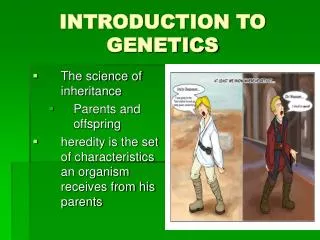
Mendel • Mendel (1865), Experiments in Plant Hybridization • No impact, paper essentially ignored • Ironically, Darwin had an apparently unread copy in his library • Why ignored? Perhaps too mathematical for 19th century biologists • The rediscovery in 1900 (by three independent groups) • Mendel’s key idea: Genes are discrete particlespassed on intact from parent to offspring

Mendel’s experiments with the Garden Pea 7 traits examined

Mendel crossed a pure-breeding yellow pea line with a pure-breeding green line. Let P1 denote the pure-breeding yellow (parental line 1) P2 the pure-breed green (parental line 2) The F1, or first filial, generation is the cross of P1 x P2 (yellow x green). All resulting F1 were yellow The F2, or second filial, generation is a cross of two F1’s In F2, 1/4 are green, 3/4 are yellow This outbreak of variation blows the theory of blending inheritance right out of the water.

Mendel also observed that the P1, F1 and F2 Yellow lines behaved differently when crossed to pure green P1 yellow x P2 (pure green) --> all yellow F1 yellow x P2 (pure green) --> 1/2 yellow, 1/2 green F2 yellow x P2 (pure green) --> 2/3 yellow, 1/3 green

Mendel’s explanation Genes are discrete particles, with each parent passing one copy to its offspring. Let an allele be a particular copy of a gene. In Diploids, each parent carries two alleles for every gene Pure Yellow parents have two Y (or yellow) alleles We can thus write their genotype as YY Likewise, pure green parents have two g (or green) alleles Their genotype is thus gg Since there are tons of genes, we refer to a particular gene by given names, say the pea-color gene (or locus)

Each parent contributes one of its two alleles (at random) to its offspring Hence, a YY parent always contributes a Y, while a gg parent always contributes a g An individual carrying only one type of an allele (e.g. yy or gg) is said to be a homozygote In the F1, YY x gg --> all individuals are Yg An individual carrying two types of alleles is said to be a heterozygote.

The phenotype of an individual is the trait value we observe For this particular gene, the map from genotype to phenotype is as follows: YY --> yellow Yg --> yellow gg --> green Since the Yg heterozygote has the same phenotypic value as the YY homozygote, we say (equivalently) Y is dominant to g, or g is recessive to Y

Explaining the crosses F1 x F1 -> Yg x Yg Prob(YY) = yellow(dad)*yellow(mom) = (1/2)*(1/2) Prob(gg) = green(dad)*green(mom) = (1/2)*(1/2) Prob(Yg) = 1-Pr(YY) - Pr(gg) = 1/2 Prob(Yg) = yellow(dad)*green(mom) + green(dad)*yellow(mom) Hence, Prob(Yellow phenotype) = Pr(YY) + Pr(Yg) = 3/4 Prob(green phenotype) = Pr(gg) = 1/4

Review of terms (so far) • Gene • Locus • Allele • Homozygote • Heterozygote • Dominant • Recessive • Genotype • Phenotype

Prob(F2 yellow is Yg) = Pr(yellow | Yg)*Pr(Yg in F2) Pr(Yellow) In class problem (5 minutes) Explain why F2 yellow x P2 (pure green) - -> 2/3 yellow, 1/3 green F2 yellows are a mix, being either Yg or YY = (1* 1/2)/(3/4) = 2/3 2/3 of crosses are Yg x gg -> 1/2 Yg (yellow), 1/2 gg (green) 1/3 of crosses are YY x gg -> all Yg (yellow) Pr(yellow) = (2/3)*(1/2) + (1/3) = 2/3

Dealing with two (or more) genes For his 7 traits, Mendel observed Independent Assortment The genotype at one locus is independent of the second RR, Rr - round seeds, rr - wrinkled seeds Pure round, green (RRgg) x pure wrinkled yellow (rrYY) F1 --> RrYg = round, yellow What about the F2?

Let R- denote RR and Rr. R- are round. Note in F2, Pr(R-) = 1/2 + 1/4 = 3/4 Likewise, Y- are YY or Yg, and are yellow Or a 9:3:3:1 ratio

Probabilities for more complex genotypes Cross AaBBCcDD X aaBbCcDd What is Pr(aaBBCCDD)? Under independent assortment, = Pr(aa)*Pr(BB)*Pr(CC)*Pr(DD) = (1/2*1)*(1*1/2)*(1/2*1/2)*(1*1/2) = 1/26 What is Pr(AaBbCc)? = Pr(Aa)*Pr(Bb)*Pr(Cc) = (1/2)*(1/2)*(1/2) = 1/8

Mendel was wrong: Linkage Bateson and Punnet looked at flower color: P (purple) dominant over p (red ) pollen shape: L (long) dominant over l (round) Excess of PL, pl gametes over Pl, pL Departure from independent assortment

Interlude: Chromosomal theory of inheritance Early light microscope work on dividing cells revealed small (usually) rod-shaped structures that appear to pair during cell division. These are chromosomes. It was soon postulated that Genes are carried on chromosomes, because chromosomes behaved in a fashion that would generate Mendel’s laws. We now know that each chromosome consists of a single double-stranded DNA molecule (covered with proteins), and it is this DNA that codes for the genes.

Humans have 23 pairs of chromosomes (for a total of 46) 22 pairs of autosomes (chromosomes 1 to 22) 1 pair of sex chromosomes -- XX in females, XY in males Humans also have another type of DNA molecule, namely the mitochondrial DNA genome that exists in tens to thousands of copies in the mitochondria present in all our cells mtDNA is usual in that it is strictly maternally inherited. Offspring get only their mother’s mtDNA.

Linkage If genes are located on different chromosomes they (with very few exceptions) show independent assortment. Indeed, peas have only 7 chromosomes, so was Mendel lucky in choosing seven traits at random that happen to all be on different chromosomes? Problem: compute this probability. However, genes on the same chromosome, especially if they are close to each other, tend to be passed onto their offspring in the same configuation as on the parental chromosomes.

Consider the Bateson-Punnet pea data Let PL / pl denote that in the parent, one chromosome carries the P and L alleles (at the flower color and pollen shape loci, respectively), while the other chromosome carries the p and l alleles. Unless there is a recombination event, one of the two parental chromosome types (PL or pl) are passed onto the offspring. These are called the parental gametes. However, if a recombination event occurs, a PL/pl parent can generate Pl and pL recombinant chromosomes to pass onto its offspring.

Recombinant gametes in deficiency, as c/2 < 1/4 for c < 1/2 Parental gametes in excess, as (1-c)/2 > 1/4 for c < 1/2 Let c denote the recombination frequency --- the probability that a randomly-chosen gamete from the parent is of the recombinant type (i.e., it is not a parental gamete). For a PL/pl parent, the gamete frequencies are

Expected genotype frequencies under linkage Suppose we cross PL/pl X PL/pl parents What are the expected frequencies in their offspring? Pr(PPLL) = Pr(PL|father)*Pr(PL|mother) = [(1-c)/2]*[(1-c)/2] = (1-c)2/4 Likewise, Pr(ppll) = (1-c)2/4 Recall from previous data that freq(ppll) = 55/381 =0.144 Hence, (1-c)2/4 = 0.144, or c = 0.24

Generally, to compute the expected genotype probabilities, need to consider the frequencies of gametes produced by both parents. Suppose dad = Pl/pL, mom = PL/pl Pr(PPLL) = Pr(PL|dad)*Pr(PL|mom) = [c/2]*[(1-c)/2] Notation: when PL/pl, we say that alleles P and L are in cis When parent is Pl/pL, we say that P and L are in trans

The Prior Probability of Linkage Morton (1955), in the context of linkage analysis in humans, introduced the concept of a Posterior Error Rate, or PER PER = probability that a test declared significant is a false positive, PEF = Pr(false positive | significant test) The screening paradox: type I error control may not lead to a suitably low PER With PER, conditioning on the test being significant, As opposed to conditioning on the hypothesis being a null, as occurs with type I error control (a)

Pr(false positive | null True )* Pr(null) PER = Pr(significant test) Let a be the Type 1 error, b the type 2 error (1- b = power) And p be the fraction of null hypothesis, then from Bayes’ theorem PER = Pr(false positive | significant) Since there are 23 pairs of human chromosomes, Morton argued that two randomly-chosen genes had a 1/23 (roughly 5%) prior probability of linkage, i.e. p = 0.95

0.05*0.95 = 0.54 0.05*0.95 + 0.8*0.05 Assuming a type I error of a = 0.05 and 80% power (b = 0.2), the expected PER is Hence, even with a 5% type-I error control, a random significant test has a 54% chance of being a false-positive. This is because most of the hypotheses are expected to null. If we draw 1000 random pairs of loci, 950 are expected to be unlinked, and we expect 950 * 0.05 = 47.5 of these to show a false-positive. Conversely, only 50 are expected to be linked, and we would declare 50 * 0.80 = 40 of these to be significant, so that 47.5/87.5 of the significant results are due to false-positives.

Genes and DNA

Structure of DNA Deoxyribonucleic Acid(DNA) Very long polymer of four bases Adenine (A) Guanine (G) Thymine (T) Cytosine (C) Key: DNA is a double-stranded molecule with complementary base-pairing A pairs with T G pairs with C

The DNA helix consists of two anti-parallel strands

DNA vs. RNA DNA -- codes for the genes. Stable and biologically inert. RNA = Ribonucleic Acid . Has the 2’OH group that DNA (deoxy-RNA) lacks. The T base is replace by Uracil, U This 2’OH group makes RNA a potentially very active molecule. RNAs involved in several features of basic cellular metabolism mRNA, tRNA, rRNA Single-stranded but with lots of secondary structure

2’ OH group lacking in DNA

Regulatory regions (enhancers and suppression) may lie at a good distance from the gene Basic structure of a Gene A region of DNA is transcribed into an RNA molecule

The Central Dogma DNA -> RNA -> proteins Translation, occurs on ribosomes

Regulation of Gene expression Can occur by controlling translation (making RNA) At transcription (RNA -> protein) Post-transcriptional (proteins may exist in non-functional stages that must be processed to be active. Example: blood clotting factors.) Importance of gene and regulatory networks

Molecular Markers DNA is highly polymorphic Roughly one in every 100 to 1,000 bases differs between otherwise identical genes. Two randomly-chosen humans differ at roughly 20,000,000 bases These polymorphic sites serve as abundant genetic markers for mapping and gene discovery

----ACACACAC ---- Variation at a STR ----ACACACACACAC ---- Types of molecular markers SNP = Single Nucleotide Polymorphisms SNP usually consists of only two alleles STR = Simple Tandem Arrays STR (also called microsatellites) can have a very large number of alleles and hence be highly polymorphic. This makes then excellent for many mapping studies.

Introduction to Genetics