Download
1 / 77
770 likes | 1.06k Vues
Network Measurement for Wide-area Load Balancing C. Edward Chow. Outline of the Talk. Introduction Why we measure What to measure Problems faced by Internet network measurement Taxonomy of Internet network measurement techniques New measurement techniques

E N D
Network Measurement for Wide-area Load BalancingC. Edward Chow C. Edward Chow
Outline of the Talk • Introduction • Why we measure • What to measure • Problems faced by Internet network measurement • Taxonomy of Internet network measurement techniques • New measurement techniques • How to apply them in WAN load balancing C. Edward Chow
Server2 Server8 Server9 Server1 router router router router Internet Environment router router Internet client C. Edward Chow
Which one do I choose? Netscape software mirror sites in Japan Download: Japan, Japan Advanced Institute of Science and Technology Download: Japan, Hokkaido University Download: Japan, International University of Japan Download: Japan, Kyushu University Download: Japan, SunSITE Japan (Science University of Tokyo) Download: Japan, Toyama Prefectural University C. Edward Chow
Oops! I Forgot It Was Updated Chris, The bprobe testing data on the 512Kbps fraction T1 connection to www.westgov.org indicates that the link has 1.49Mbps bandwidth (close?) and the cprobe testing data on it indicates that the link has about 793kbps available bandwidth, which is different from 512Kbps number. (Very disappointed!!) -Edward “Ahh - it got upgraded. Try: mwrd.dst.co.us It's a fractional T1, but I'll let you figure out how many channels. Treno reports this one pretty well (but it's as intrusive as these things get).” -Chris (cgarner@sni.net)” C. Edward Chow
How much buffer I need for Internet[V|A]udio? • Real-time continuous multimedia applications need to tolerate and adapt to Internet network delay and jitter. • Through error concealment (drop late packets) or destination buffering and adjusting application parameter (packet rate and resolution). • By continuous monitoring directional path delay/jitter • Example: RTP, Realplayer, InternetPhone C. Edward Chow
Why Measure? • Measurement is the basic [and prelude] of control. -Tsueno Katsuyama • Measurement for selecting server/ISP/equipment. • Measurement for verifying network configuration. • Measurement for designing Internet applications • Measurement for configuring network/servers • Measurement for load balancing in WAN • Measurement for accounting $$ C. Edward Chow
What to Measure? • Performance of network systems involves • server performance • network path performance • client performance • Reachability • Packet Delay (One way or round trip?) • Hop count • Available bandwidth (uni-directional or bi-directional?) • Bottleneck bandwidth • Packet Loss Rate C. Edward Chow
IP header 20 B ethernet header 14 B ICMP header 8 B Measure Round Trip Delay • Ping can be used to measure the reachability and round trip delay. • Sender sends ICMP echo request (Type=8) msg to the receiver with sending timestamp in data field. • Receiver replies with ICMP echo reply (Type=0) msg. • Round trip delay = arrival time - sending_timestamp • 64 bytes from 128.198.66.37: icmp_seq=0 ttl=30 time=331.5 ms13 packets transmitted, 12 packets received, 7% packet lossround-trip min/avg/max = 241.9/260.7/331.5 ms Type 1B chksum 2B code 1B ID 2B Seq# 2B Timestamp 4B ICMP option data C. Edward Chow
Measure Unidirectional Delay • Modified Ping by Kimberly Claffy, George C. Polyzos, Hans-Werner Braun, UCSD • Send ICMP time-stamp request packets to destinationwith its current time value in “originate timestamp” field • Destination puts receiving timestamp field value when receives. • Destination puts its current time into transmit timestamp field when replies • Outbound delay = receiving timestamp - originate timestampReturn delay = arrival timestamp - transmit timestamp C. Edward Chow
Examples: Assessing Unidirectional Latencies From San Diego to scslwide.sony.co.jp C. Edward Chow
Difficulties and Anomalies in Internet Network Measurement • Packet Loss • Clock Resolution/Synchronization • Routing Pathologies: Wrong TTL in reply, out-order delivery, duplicate packets • Route Asymmetry/Change/Flattering • Congested router with multiple interface • Routing in Link Layer • Firewall, ICMP reply rate control. • Link adjust bandwidth according to traffic C. Edward Chow
Clock Resolution/Synchronization • Outbound delay = receiving timestamp - originate timestamp depend on clock values at the source and destination sites. • Clock drifts 3 - 60 msec per hour on workstations. • Synchronize the clocks on two sites by NTP or GPS. • NTP can adjust clock difference < 10 msec [Miller92] • GPS resolution much higher? • Is the clock resolution good enough? • Claffy’s study focus on asymmetric delay variance. Their values 1 or 2 order magnitude larger clock difference • Increase size of Timestamp(4B->8B). NTP 20xx problem. C. Edward Chow
Time Travel [Paxon97] Back to the past! How about back to the future? C. Edward Chow
Route Flattering • fluttering -- rapidlyvariable routingmost for load balancing reason? Here is a traceroute result: 8 nationalaixus.gw.au 1039 ms * * 9 * rb1.rtr.unimelb.edu.au 903 ms rb2.rtr.unimelb.edu.au 1279 ms 10 itee.rtr.unimelb.edu.au 1067 ms 1097 ms 872 ms • 9th hop alternates between rb1 and rb2 of rtr.unimeb.edu.au (8th hop could be changed also) C. Edward Chow
Bottleneck Bandwidth Change[Paxon97] ISDN line 13.3kB/s 6.6kB/s C. Edward Chow
Multichannel Effect 160kB/s 13.3kB/s C. Edward Chow
Hourly Variation Ack Loss RateNorth America [Paxon97] C. Edward Chow
Hourly Variation Ack Loss RateEurope C. Edward Chow
Dealing with those problems • Use burst of probing packets to avoid packet loss. • Use sequence # to detect out-of-order delivery, duplicate packets. • Use traceroute to detect route change/flutter (very expensive) C. Edward Chow
Taxonomy of Internet Network Measurement Approaches • Sender-based vs. Receiver-based • Packet Pair vs. Packet Bunch • Point-to-Point vs. Multipoint • Passive Watch vs. Active Probe • Cooperative (Shared) vs. Isolated • Layer of Protocol used • On-line vs. Off-line • Long term vs. Short term • Localized vs. Network wide C. Edward Chow
Sender-Based vs. Receiver-Based • Sender-based relies on the receiver to reply or echo sender’s packets. Ping, Traceroute, Bprobe/Cprobe • Does not require special access on the receiver site. • Measurement related to round trip, two directional paths, difficult separate the contribution. • Receiver-based requires cooperation (time calibration/synchronization) and access to both ends. • Measure uni-directional path data. NPD • Characteristics on two directional paths can be quite different [Paxon97] C. Edward Chow
Packet Pair vs. Packet Bunch • Specific referred to bottleneck bandwidth measurement • Packet Pair measures gap between two packets. • Packet Bunch measures k (k>2) packets as a group • Deal with low clock resolution. For clock resolution Cr=10 msec and packet size 512 byte, packet pair cannot distinguish between 512/0.01=51.2kB/s and infinite • Deal with changes in bottleneck bandwidth • Deal with multi-channel links C. Edward Chow
Point-to-Point vs. Multipoint • Point-to-point involves two end points in isolated measurements. • Multipoint involves multiple end points in cooperative measurements. • For link connected to busy router with many interfaces, multipoint measurement may be the only way to avoid interference traffic. • Multipoint measurement is a new area worth exploring. C. Edward Chow
Passive Watch vs. Active Probe • In passive watch, measuring machine observe and measure passing traffic. • No probing traffic to overload the network. • Fujitsu SmartScatter • ARPwatch and RIPwatch module in Fremont system. • Katz’s Shared Passive Network Performance Discovery (SPAND) • What happens if there is no traffic? • Does it require special instrumentation or protocol change? C. Edward Chow
SPAND [UCB-CSD-97-967] C. Edward Chow
Cooperative (Shared) vs. Isolated • The network measurement results to a remote site should be the similar for all the hosts in the subnet. • By sharing the information, the redundant probing traffic can be eliminated. • SPAND is cooperative but passive watch. • The Multipoint measurement example mentioned is cooperative but active probe. C. Edward Chow
Layer of Protocol Used • The use of lower layer protocol enables more timing and programming control. • The measured throughput reflects the upper bound of the predict traffic if higher layer protocol are used. • The use of higher layer protocol such as http or ftp reflects more accurate the performance but requires complex analysis to be used for other application traffic. • Ping uses ICMP. Traceroute uses UDP and ICMP. • NPD uses TCP but forgot to keep track ICMP src quench msgs. C. Edward Chow
Measure Internet Link Speed • Bob Carter and Mark E. Crovella’s work (Boston U.) • Bprobe estimates bottleneck link speed of a path • Cprobe estimates available bandwidth of a path • use short burst of ICMP echo packets • use time gaps between ICMP echo reply to infer the bandwidth • use filter to weed out inaccurate measurements • Matt Mathis’s work (Pittsburgh Supercomputer Center) • Treno emulate TCP Reno Congestion Control • use UDP, require 10 seconds of continuous traffic C. Edward Chow
Bprobe and Cprobe • Discuss the theory behind them • It was originally design on SGI using 40ns hardware clock. • It was ported to Linux PC using gettimeofday(). • Several significant bugs were detected and fixed. • Present preliminary testing results and code assessment. C. Edward Chow
Packet Flow Through a Bottleneck Link (Van Jacobson) estimated bandwidth = P/Dt P bytes Dt C. Edward Chow
Obstacles and Solutions to Measuring Base Bandwidth • Queuing Failure. Not fast enough to cause queuing at the bottleneck router. • send a short burst of packets (e.g., 10) • send larger size packets (124, 186, 446, 700, 1750, 2626, 6566) • starting with 124 gradually increase the size • why 124? why 10? C. Edward Chow
Obstacles: Competing Traffic C. Edward Chow
Solution to Competing Traffic • Sending a large number of packets and increase the probability that some pairs will not be interleaving with competing traffic. • Intervening packet size often varies. Use filter to rule out incorrect estimates. • Alternating the increase of packet size (1.5 and 2.5) to reduce the probability of bad estimate.even(124*1.5)=186, even(186*2.5)=446,even(445*1.5)=700, even(700*2.5)=1750even(1750*1.5)=2626, even(2626*2.6)=6566 • Why even? why 1.5 and 2.5? C. Edward Chow
Obstacles and Solutions for Measuring Based Bandwidth • Probe Packet Drop. Large packet more likely to cause buffer overflow and be dropped.Avoid by sending packets of varying sizes. • Downstream Congestion. On returning trip the gap generated by bottleneck link may be reduced if there is a congestion between the bottleneck link and the source.If enough of pairs return without further queuing, the erroneous estimates can be filtered out. C. Edward Chow
Samples of Measurements C. Edward Chow
Filtering Process arrival gap size error interval or bin size, dynamic adjust until reasonable # of bin reached estimated bandwidth union(Set1,Set2) estimated bandwidth intersection(Set1,Set2) C. Edward Chow
Histogram of Bprobe Results 56kbps hosts on NearNet A region network C. Edward Chow
Histogram of Bprobe Results T1 Hosts on NearNet Not as accurate as 56kbps C. Edward Chow
Histogram of Bprobe Results Ethernet Hosts on NearNet C. Edward Chow
Accuracy of Bprobe C. Edward Chow
Bprobe* Test on Sni.net • Here use the ported bprobe without high resolution hardware clock and setting higher process priority. Chris, The bprobe testing data on the 512Kbps fraction T1 connection to www.westgov.org indicates that the link has 1.49Mbps bandwidth (close?) and the cprobe testing data on it indicates that the link has about 793kbps available bandwidth, which is different from 512kbps number. (Very disappointed!!) C. Edward Chow
Bprobe* Exam on Sni.net “Ahh - it got upgraded. Try: mwrd.dst.co.us It's a fractional T1, but I'll let you figure out how many channels. Treno reports this one pretty well (but it's as intrusive as these things get). -Chris (cgarner@sni.net)” • What this says about the accuracy of network configuration query? • Suddenly there is still hope for bprobe. C. Edward Chow
Am I right? “The bottleneck bandwidth from gandalf.uccs.edu to mwrd.dst.co.us is 108465.5 bps. The available bandwidth is about 98062.5734376. I would say this fractional T1 has two DS0 slots 64*2=128 kbps (a bit off from estimated bandwidth) or 56*2=112 kbps (closer some runs indicate 111201 bps). Am I right? -- Edward” C. Edward Chow
Bprobe* Test on 56kbps bprobe canon.k12.co.us 10 times (*: The ported version of Bprobe) trial# bottleneck_bw 0 5.21880e+04 1 5.76160e+04 2 5.11160e+04 3 5.35500e+04 4 5.64610e+04 5 5.21760e+04 6 5.27600e+04 7 5.23460e+04 8 5.33370e+04 9 5.58370e+04 valid trial#=10, average bottleneck bw=53738.7 C. Edward Chow
bprobe 206.251.6.35 20 times trial# bottleneck_bw 0 1.53498e+06 1 1.80729e+06 2 2.73521e+06 3 1.83016e+06 4 1.51497e+06 5 1.52228e+06 6 1.51137e+06 7 1.53590e+06 8 1.48853e+06 9 1.49629e+06 10 1.44828e+06 11 1.49212e+06 12 1.52818e+06 13 1.48306e+06 14 1.56945e+06 15 2.37321e+06 16 1.53305e+06 17 1.09638e+06 18 1.53427e+06 19 1.52435e+06 valid trial#=20, average bottleneck bw=1627966.5 Bprobe* Test on T1 Line C. Edward Chow
Cprobe • Bounce a short burst of ICMP Echo Packet off Server • Bavail = Length_of_Short_Burst/(Tlast_pkt -T1st_pkt) • Utilization of the bottleneck link:Uprobe = Bavail/Bbls where Bbls are measurement of bottleneck link bandwidth • The above definition contradicts the traditional way that define the utilization (the port being used) • They throw away the highest and lowest inter-arrival measurement for more accurate results. C. Edward Chow
Fractile Quantities of Cprobe’s Available Bandwidth Estimates* * These results were obtained using the packet trace tool on a local Ethernet . C. Edward Chow