Pendulum Mock Lab
Pendulum Mock Lab. Part 1: Experimental Design. Focused Research Question:. I will investigate how the period of a pendulum depends on its length. Variables:. Independent - L = length of the pendulum string (m) Dependent - t = time for one swing (s)


Pendulum Mock Lab
E N D
Presentation Transcript
Part 1: Experimental Design Focused Research Question: I will investigate how the period of a pendulum depends on its length Variables: Independent - L = length of the pendulum string (m) Dependent - t = time for one swing (s) Controlled - angle of swing (degrees), mass of the bob (g), Equipment: Ceiling hook, string, hanging mass, stopwatch, electronic scale, protractor, meter stick marked in mm, scissors, paper
Part 1: Experimental Design Method: The hook is attached to the ceiling and string is cut to make ten lengths differing by 25cm from over two meters in length to under half a meter in length. The pendulum bob is massed and the string is tied to the ceiling hook at one end and to the bob at the other. The distance from the pivot position at the hook to the center of the bob is taken as the pendulum length. The angle of swing is set at five degrees. To do this repeatedly, a sheet of paper is marked with a vertical plumb line and five degrees is marked with reference to that line. The paper is taped to the ceiling behind the string when in its relaxed vertical position. The bob is pulled back from it’s relaxed position to five degrees and the timer is started on release. The time for five complete back and forth motions of the pendulum bob is recorded. This is repeated three times. The pendulum is then adjusted for a new length and the process is repeated.
Part 2: Data Collection and Processing Data Table: Identifying, specific title Multiple tables must be numbered Table 1. Length vs. Period For a Pendulum Mass of the pendulum bob is 103 1 g The angle of swing is 5 1 degrees Constants are listed above the table Units given per measured quantity Uncertainty recorded to 1 SF Appropriate data set Large spread of data
Processing Raw Data: (Example calculations put under the data table) Determining the period: Average for 5 cycles = time1 + time2 + time3 3 = 14.3 s + 14.4 s + 14.4 s = 14.4 s 3 Period = Av. Time for 5 swings 5 = 14.4 s = 2.9 ± 0.1 s 5 Calculated uncertainty in the period: T = t / number of swings = 0.6 s / 5 = 0.1 s
Full descriptive title Graph: Curve-fit your data No dot-to-dot Axes labels with units Data, column options, options to select error bars Type in value Using (0,0) shows data does not fit a straight line
Language of physics - Uncertainties in Graphs Because all data contains uncertainties at the very least data points should be marked as small circles or crosses. If the absolute uncertainty in each measurement is known then uncertainty bars should be used to turn the data point into a data area. Never connect data points “dot to dot”.
Language of physics - Graphs (recognizing functions) So you’ve found a question that needs to be answered, identified variables, restricted them, produced a mathematical model and devised an experiment that will collect data. How do you know that your data supports or refutes your model? The answer lies in graphs – It is important to be able to recognize the shape of a graph and be able to relate that shape to a mathematical function. You can then compare this function to your model. Some functions found in physics are shown on the next two slides! Direct yx y = kx k = slope of the line y is directly proportional to x Note: If the line does not go through (o,o) it is linear y = kx + b b = y intercept Independent y = k y does not depend on x b
Language of physics - Graphs (recognizing functions) Inverse Proportional y 1/x y = k/x y = k x-1 y is inversely proportional to x Square yx2 y = kx2 y is proportional to the square of x Square root y √x y = k √ x Y = k x1/2 Y is proportional to the square root of x Note: all these functions are all power functions as they fit the general expression, y = A xBwhere A and B are constants
Language of physics - Graphs (recognizing functions) Exponential Growth y = anbx y increases exponentially with x Exponential Decay y = an−bx Y decreases exponentially with x Periodic y = A sin (Bx + C) Y varies periodically with x
Language of physics - Graphs (recognizing functions) Let’s say that you are investigating how the period (T) of a pendulum (time for one swing) depends on the length (l) of the pendulum and you have come up with a mathematical model that says, T = 2 ( L/ g). You then test this model experimentally and plot a graph of T vs. L (shown below). Which function best describes your data? The curve through the data can’t be a straight line because as the length decreases, the period decreases so at zero length we would expect the pendulum to take no time to swing back and forth. The model says that T L or T L1/2 This suggests that we should look at a power function and in particular a square root function (y=kx1/2) You can see that the computer generated power function fit is a good fit to our model as the data fits T = (2.06) L0.44 The power 0.44 is close to 0.5 (1/2) We can also use our data to verify the constant g because Comparing our model with the fit equation we find 2 / g = 2.06 so g = (2 / 2.06)2 = 9.3
Language of physics - Graphs (turning a curve into a straight line) Sometimes its nicer to see a relationship from a straight line graph rather than a curved graph, especially when we use uncertainty bars (next slide). To turn a curve into a straight line you look at the proportional statement. If you wanted to turn the pendulum curved graph into a straight line graph what would you plot on each axis? Now T L so our data should fit a straight line if we plot T vs. L instead of T vs. l Processing Raw Data: Length = (2.15m) = 1.47 m1/2
Straight Line Graph: You can see that the data now fits a nice straight line The slope (1.8) can be related back to the proportionality constant which is 2 / g
Analyzing Straight Line Graph: The graph opposite shows possible slopes within an uncertainty range We can easily sketch the best-fit line (black) and the two worst (min slope (blue) and the max slope (green)) acceptable lines by using the extremes of the uncertainty bars on the first and last points. The graph thus performs the function of averaging the data.
Determining uncertainty in the slope: Determining max slope: mmax = (Tmax + T) – (Tmin - T) Lmax1/2 – Lmin1/2 = (2.9s+0.1s) – (1.3s-0.1s) (1.47 m1/2 – 0.59 m1/2) mmax = 1.8 s / 0.88 m1/2 = 2.0 sm-1/2 Determining min slope: mmin = (Tmax - T) – (Tmin + T) Lmax1/2 – Lmin1/2 = (2.9s-0.1s) – (1.3s+0.1s) (1.47 m1/2 – 0.59 m1/2) mmin = 1.4 s / 0.88 m1/2 = 1.6 sm-1/2 So slope of the graph is 1.8 ± 0.2 sm-1/2
Part 3: Conclusion and Evaluation Concluding: The slope of the graph represents 2 / g gmax = (2 / mmin)2 = (2 / 1.6 sm-1/2)2 = 15 m/s2 gmin = (2 / mmax)2 = (2 / 2.0 sm-1/2)2 = 9.9 m/s2 gfit = (2 / m)2 = (2 / 1.8 sm-1/2)2 = 12 m/s2 gactual = 9.81 m/s2 g can thus be quoted as 12 ± 3 m/s2. The actual value of g (9.81 m/s2) is within this range. It can be seen that small differences in the slope can lead to large differences in the value of g because of the squaring operation.
Part 3: Conclusion and Evaluation Concluding: I’ll show you another way another way of determining g without using graphical interpretation. This method is limited in that it is based on one point and so doesn’t reflect the range of your data. From your table choose a mid point, L = 115 ± 1cm, T = 2.2 ± 0.1s. T = 2(L/g) so…. g = L (2 / T)2 so…. gav = L (2 / T)2 = (1.15m) (2 / (2.2s))2 = 9.4 m/s2 Using uncertainty rules for multiplication and powers…. g / g = L / L + 2 (T / T) = (1 / 115) + 2 (0.1 / 2.2) = 0.0996 g = (0.0996) x g = (0.0996) x 9.4 m/s2 = 0.93 m/s2 gav can thus be quoted as 9.4 ± 0.9 m/s2. The actual value of g (9.81 m/s2) is within this range.
Part 3: Conclusion and Evaluation Concluding: You can calculate a percentage difference between the accepted value of g and your calculated average value using.. This shows a good correlation but it doesn’t reflect the larger range in possible values of g that 12 ± 3 m/s shows.
Part 3: Conclusion and Evaluation Concluding: The direction of systematic errors Looking at the Period vs. Square Root of the Length Graph, it can be seen that the best-fit line does not go through the origin, (0,0). It gives a positive y intercept. If the slope (gradient) was steeper, gfit would have been smaller than 12 m/s2. If the string length was measured before being hung from the ceiling support with the mass attached, the mass could have stretched the string giving rise to a systematic uncertainty in the length of the string. This would be more significant for shorter lengths.
Part 3: Conclusion and Evaluation Evaluating Procedure(s): Although the mass of the pendulum bob should not be a factor in this experiment, air drag on the string and bob might increase the period of swing thus giving a non-zero y intercept on the straight-line graph. Timing the swing time of shorter pendulum lengths gives a larger uncertainty in determining g than for longer lengths. String lengths are limited by the height of the room.
Part 3: Conclusion and Evaluation Improving the Investigation: Use of as thin a string as possible, such as fishing line and a lead weight as the bob with large mass and small volume should offer the least amount of aerodynamic drag. To reduce reaction-time random uncertainties, a photogate timer may be used at the bottom of the pendulum swing. Again, a series of swings should be timed and the average time for one swing should be determined The string length should be measured after the bob is mounted before and after taking a series of measurements. A higher ceiling room giving rise to longer pendulum lengths would reduce the effects of uncertainty in L and t but swinging through more air would cause drag to factor more.