FFT corrections for tune measurements
210 likes | 462 Vues
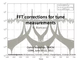
FFT corrections for tune measurements. N. Biancacci. Optics Workshop, OMCM CERN, June 20-22, 2011. Acknowledgements: M.Giovannozzi, F.Schmidt , E.Métral, Y.Papaphilippou , B.Salvant, R.Tomás. Discrete F ourier T ransform (DFT) on harmonic signals FFT- ApFFT - FFTc -NAFF-SUSSIX

FFT corrections for tune measurements
E N D
Presentation Transcript
FFT corrections for tune measurements N. Biancacci Optics Workshop, OMCM CERN, June 20-22, 2011 Acknowledgements: M.Giovannozzi, F.Schmidt, E.Métral, Y.Papaphilippou , B.Salvant, R.Tomás.
Discrete Fourier Transform (DFT) on harmonic signals FFT-ApFFT-FFTc-NAFF-SUSSIX Comparisons between different methods to achieve higher resolutions in amplitude, frequency and phase advance. Conclusions and outlook Outline 1/17
DFT on harmonic signals BPM ADC Noise + Memory 2/17
Continuum case: DFT on harmonic signals 3/17
Discrete case: Having a finite number of samples corresponds to windowing with a “rect” function r[n] the sampled signal. DFT on harmonic signals This operation is a convolution in the discrete frequency domain. Applying the DFT formula on r[n] and applying translation property* from s[n], we get: 4/17 * DFT translation property
Observations: DFT on harmonic signals Frequency shiftAmplitude distortion Phase shift Naming where m is the index corresponding to the highest peak in amplitude spectrum, one can see that Amplitude, phase and frequency resolutions depend on the error δ in localizing the spectrum maximum. Resolution in frequency is related to the length of samples but also to the value of δ (correspond to the real value if δ=0). Without correction, making the phase basically useless. Resolution in amplitude is dependent from the resolution in frequency and the window shape. 5/17 m
To overcome these limits and recover the real parameters for the harmonic signals different methods were proposed*: FFTc ‘Corrected FFT’ Used to correct the amplitude, phase and frequency. Based on analytical properties of windowing functions. ApFFT ‘All phase - FFT’ Used to improve the phase resolution. Based on properly preprocessing the measured signal in order to cancel phase errors. Sussix Used to improve frequency resolution. Based on iterative routines to get the frequency of the tune. NAFF Used to improve frequency, amplitude and phase resolution. Based on iterative routines to get the tune frequency. DFT on harmonic signals In the following we present comparisons between these methods. 6/17 * All references at the end of the presentation
Using a “rect” window we get a “sinc” shape in frequency domain. This window has a nice property if one computes the baricentre for two points in the main lobe of the sinc. Corrected FFT Take the continuum function . Take two points P1(x1,y1) and P2(x2,y2) in the main lobe. The baricentre is given by: If then: It follows that P1 P2 Since in spectral analysis, k-samples are spaced by unity, taking the shifted-maximum and the second maximum, and computing the baricentreXc we get the exact position corresponding to the real maximum: 7/17
Applying the baricentre method we can get the correction formula both for “rect” and Hanning window: Rect window Hanning window Corrected FFT m m-1 m+1 m m-1 m+1 8/17
This is a preprocessing algorithm developed to correct the phase got out from the DFT operation. The computed phase is the central phase, i.e. the one corresponding to the central sample in case of an odd number of samples. ApFFT Multiply the signal with a triangular window: Fold the windowed signal: Proceed to FFT evaluation and extract the phase: The phase is no more dependent on δ, i.e. doesn’t need to be corrected. 9/17
The NAFF code was developed by J.Laskar et al. in the Nineties as a method to analyze chaotic dynamical system by Numerical Analysis of the Fundamental Frequencies in the sampled signal. NAFF-Sussix Signal: The FFT is used as a “first guess seed” for the quadratic interpolation routine. FFT The interpolation routine finds the peak of moving around the expected peak. At the maximum we get the complex amplitude After a Gram-Schmidt normalization the detected harmonic is subtracted by the original signal. The method in SUSSIX and NAFF are similar. In SUSSIX it is based on the TUNEWT algorithm developed by A.Bazzani (University of Bologna) in the mid-Nineties and further developed and tested at CERN. 10/17
Different simulations were set up on detecting phase, amplitude and frequency using the different methods presented previously. In order to properly compare the phase accuracy, the phase difference between two signals at the same frequency will be analyzed. In real life the absolute phase has no sense cause to the decoherence in the signal. Comparisons All the simulations are set in presence of noise. The level is set in terms of 1-sigmaof noise. We consider the case of absence of noise (simulation case) and 1% and 10% additive gaussian noise. No noise 1% noise 10% noise 11/17
No noise Frequency VS Turns • Both FFTcand Sussix have Hanning window on the signal. • The FFT is corrected with the formulae seen before. • In case of no noise, NAFF is the most accurate (1/N^3) followed by FFTc and SUSSIX (1/N^2) • In case of noise the resolution is still better than a normal FFT, but equivalent for all FFTc, SUSSIX and NAFF. 1% noise 10% noise 12/17
No noise Amplitude Vs Turns • ApFFT (as a normal FFT) doesn’t implement any amplitude correction. • The FFTcis corrected with the formulae seen before. • Without noise FFTc goes like 1/N, NAFF like 1/N^2. • In presence of noise, NAFF and FFTc presents similar behaviour going like 1/N. • Sussix is not reported since is not thought for absolute amplitude detections. 1% noise 10% noise 13/17
No noise Phase Vs Turns • This simulation is set up with a ∆φs=60⁰. • The FFTcis corrected with the formulae seen before. • Without noise, SUSSIX and a normal FFT have a similar behaviour (1/N). • ApFFT goes like NAF as 1/N^2. • FFTc reaches higher resolutions (1/N^3). • In presence of noise all the approaches give almost the same resolution (1/N). 1% noise 10% noise 14/17
No noise Phase Vs Phase advance • This simulation is set up fixing N to 512 Turns and spacing the ∆φs from ∆φs =0⁰ to ∆φs =180⁰. • In case of no noise ApFFT and the corrected FFT give higher resolution. • In case of noise, the resolution is around 10^-3 for 1% noise and 10^-2 for 10% noise. 1% noise 10% noise 15/17
SPS phase advance V-plane Impedance Localization • Localizing coupling impedance sources is possible looking to the phase advances between different BPMs positions. • The strength of the impedance is proportional to the variation of phase advance with intensity. The relation is linear. • It is important to estimate the phase advances being over the resolution limit of the FFT used. FFT FFTc Simulated phase advance Vs intensity (from 1e10 to 8e10 ppb) Standard FFT Corrected FFT 16/17
CONCLUSIONS • The problem of getting correct phase, amplitude and frequency out of a harmonic signal was analyzed: Corrected FFT, ApFFT,SUSSIX and NAFF algorithms were presented in both a theoretical and practical point of view . • For frequency measurements NAFF has the higher resolution followed by SUSSIX and FFTc. All of them become comparable in presence of low noise. • For amplitude measurements NAFF has the higher resolution followed by FFTc. Still, in presence of noise they behave the same. • For phase measurements FFTc has the higher resolution. All the methods behave the same in presence of low noise. • All the algorithms break down in presence of noise. If needed, a stronger effort in order to reduce or “clean” it should be done. • OUTLOOK • Since SUSSIX is widely used, we can improve its speed adding the analytical corrections implemented in FFTc (single shot corrections VS iterative loops). • One can improve the corrected FFT in order to detect subsequent harmonics in the betatron signal as done in the NAFF algorithm. 17/17
About NAFF • J.Laskar, C.Froeschle, A.Celletti, “The measure of chaos by the numerical analysis of the fundamental frequencies. Application to the standard mapping “ References About SUSSIX • R. Bartolini, M. Giovannozzi, W. Scandale, A. Bazzani and E. Todesco “Precise measurement of the betatron tune ” Particle Accelerators, 1996, Vol. 55, pp. [247-256] /1-10 • R.Bartolini, M.Giovannozzi, W.Scandale , A.Bazzani, E.Todesco “Algorithms for a precise determination of the betatron tune” AboutFFT corrections • X.Ming, D.Kang “Corrections for frequency, amplitude and phase in a fast fourier transform of a harmonic signal” Mechanical Systems and Signal Processing V. 10, 2, March 1996, Pages 211-221 About Ap-FFT • X. Huang, Z. Wang, L. Ren et al. “A novel High-accuracy Digitalized Measuring Phase Method” IEEE • X.Huang, Z.Wang, G.Hou “New method of estimation of phase, amplitude and frequency based on all phase FFT spectrum analysis” IEEE About general digital signal processing theory • J.G.Proakis, D.G. Manolakis “Digital Signal Processing, principles, algorithms and applications” 4th edition.