Components of illumination
950 likes | 1.2k Vues
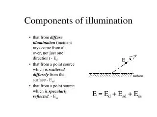
Components of illumination. that from diffuse illumination (incident rays come from all over, not just one direction) - E d that from a point source which is scattered diffusely from the surface - E sd that from a point source which is specularly reflected . - E ss. E.

Components of illumination
E N D
Presentation Transcript
Components of illumination • that from diffuse illumination (incident rays come from all over, not just one direction) - Ed • that from a point source which is scattered diffusely from the surface - Esd • that from a point source which is specularly reflected. - Ess E E = Ed + Esd + Ess
Combining the illumination • Combining all three components (diffuse illumination, diffuse reflection from a point source and specular reflection from a point source) gives us the following expression: E = Ed + Esd + Ess
Diffuse illumination • A proportion of light reaching surface is reflected back to the observer. • This proportion is derived from the angle of incident light and properties of the surface • Not dependent on the location of the viewer.
Diffuse illumination Id - incident illumination Ed - observed intensity Ed = R.Id where: • R is the reflection coefficient of the surface (0 <= R <=1) R is the proportion of the light that is reflected back out
Diffuse scattering from a point source • When a light ray strikes a surface it is scattered diffusely (i.e. in all directions) • Doesn’t change with the angle the observer is looking from
Diffuse scattering from a point source • The intensity of the reflected rays is: Esd = R.cos(i).Is i - angle of incidence – the angle between the surface normal and the ray of light - 0 <= i <= 90 Esd -intensity of the scattered diffuse rays Is - intensity of the incident light ray. R - reflection coefficient of the surface (0 <= R <=1)
Specular reflection • relationship between a ray from point source to the reflected ray is given by Lambert’s Law: i = r i - angle of incidence r - angle of reflection
Specular reflection • For a perfect reflector, all the incident light would be reflected back out in the direction of S. In fact, when the light strikes a surface it is scattered diffusely (i.e. in all directions): • For an observer viewing as an angle (s) to the reflection direction S, some fraction of the reflected light is still visible (due to the fact that the surface isn’t a perfect reflector - some degree of diffusion takes place). • How much?
Specular reflection • The proportion of light visible is a function of • the angle s (in fact it is proportional to cos(s) • the quality of the surface • angle of incidence i. • We can define a coefficient w(i) the specular reflection coefficient - which is a function of the material of which the surface is made and of i . Each surface will have its own w(i).
Specular reflection Ess = w(i).cosn(s).Is
Specular reflection • Ess is the intensity of the light ray in the direction of O • nis a fudge factor: n=1 rough surface (paper) n=10 smooth surface (glass) • w(i) is usually never calculated - simply choose a constant (0.5?). It is actually derived from the physical properties of the material from which the surface is made.
Specular reflection cosn(s) - This is in fact a fudge which has no basis in physics, (stochastic model) but works to produce reasonable results. By raising cos(s) to the power n, what we do is control how much the reflected ray spreads out as it leaves the surface.
Combining the illumination • Combining all three components (diffuse illumination, diffuse reflection from a point source and specular reflection from a point source) gives us the following expression: E = Ed + Esd + Ess
Combining the illumination E = R.Id + (R.cos(i) + w(i) + cosn(s)).Is • E is the total intensity of light seen reflected from the surface by the observer.
Calculating E • E – We’re trying to calculate E , so obviously that is unknown. • R - is defined for each surface, so we need to add it as a variable to our surface class and define it when creating the surface, so its known. • Id - The incident diffuse light - we can define this to be anything we like; 0 = darkness, for an 8-bit greyscale 255 = white. – Known • cos(i) - we can work this out from L.N • w(i) - we can define this to be anything between 0 and 1 - trial and error called for! - Known
Calculating E • n - is defined for each surface, so we need to add it as a variable to our surface class and define it when creating the surface, so, basically its known. • Is - the intensity of the incident point light source - again we can define this to be anything we like; 0 = darkness, for an 8-bit greyscale 255 = white. See below for a discussion of adding lights to our data model. - Known. • cos(s) ? Ah!
Calculating cos s • cos s = S.O • We know O • Need S
Calculating cos s • Thanks to Lambert’s law we know that S is the mirror of the incident ray about the surface normal. It can be found from some vector maths: • S = 2Q - L
Lambert Shading • Finally, we know all of the terms in the combined illumination equation and for any surface in our model we can calculate the appropriate shade. E = Rid + (R.cos(i) + w(i) + cosn(s)).Is • A program which implements this model of shading is said to implement Lambert Shading
Extending to colour • Each surface has a colour which means it reflects different colours by different amounts, i.e. it has a different value of R for red, blue and green Ered = Edred + Esdred + Essred Egreen = Edgreen + Esdgreen + Essgreen Eblue = Edblue + Esdblue + Essblue
Gouraud Shading and Phong Shading Adopted from U Strathclyde’s graphics course
Problems with Lambert • Using a different colour for each polygon means that the polygons show up very clearly (the appearance of the model is said to be facetted.
Mach bands • This is a physiological effect whereby the contrast between two areas of a different shade is enhanced as the border between the shades
Smooth Shading • What is required is some means of smoothing the sudden transition in colour. • Various algorithms exist for this; amongst the best known are: • Gouraud shading and • Phong shading • both named after their inventors.
Gouraud Shading • The facetted appearance of a Lambert shaded model is due to each polygon having only a single colour. • To avoid this effect, it is necessary to vary the colour across a polygon:
Gouraud Shading • Colour must be calculated for each pixel of the polygon. • The method we use to calculate the colour results in the neighbouring pixels across the border between two polygons ending up with approximately the same colours. • This blends the shades of the two polygons and avoids the sudden discontinuity at the border.
Gouraud shading • based upon calculating a vertex normal • an artificial construct (a true normal cannot exist for a point such as a vertexl). • can be thought of as the average of the normals of all the polygons that share that vertex
Gouraud shading • Having found the vertex normals for each vertex of the polygon we want to shade, we can calculate the colour at each vertex using the same formula that we did for Lambert Shading
Calculating the colour of each pixel • Interpolating “scan-line algorithm” • Light intensity at P given by:
Phong Shading • Phong shading is based on interpolating the surface normal vector • The arrows (and thus the interpolated vectors) give an indication of the curvature of the smooth surface which the flat polygon is approximating to.
Phong Shading • The interpolation is (like Gouraud shading) based upon calculating the vertex normals (red arrows)…. • …using these as the basis for interpolatation along the polygon edges (blue arrows) …. • …..and then using these as the basis for interpolating along a scan line to produce the internal normals (green vectors) • a colour value calculated for each pixel based on the interpolated value of the normal vector.
Gouraud vs Phong • Phong shading is requires more calculations, but produces better results for specular reflection than Goraud shading in the form of more realistic highlights.
Why? • Consider the specular reflection term Cosn s If n is large (the surface is a good smooth reflector) and one vertex has a very small value of s (it is reflecting the light ray in the direction of the observer) whilst the rest of the vertices have large values of s - a highlight occurs somewhere on our polygon.
Why? • With Gouraud shading, nowhere on the polygon can have a brighter colour (i.e higher value) than a vertex • unless the highlight occurs on or near a vertex, it will be missed out altogether. • When it is near a vertex, its effect is spread over the whole polygon. • With Phong shading however, an internal point may indeed have a higher value than a vertex. and the highlight will occur tightly focused in the (approximately) correct position
Summary • Lambert shading leads to a facetted appearance • To get round this, use a smooth shading algorithm • Gouraud and Phong shading produce good effects but at the cost of more calculations. • Gouraud interpolates the calculated vertex colours • Phong interpolates the calculated vertex normals • Phong – slower but better highlights
Finer Details • Adding fine details • Why we don’t use the brute force approach • Faking it with pictures
Fine details • We could explicitly model this block of wood with lots of small, different coloured surfaces. • Immense amount of work.
Fine details • In fact, we don’t. • “Stick” a picture (.bmp, .gif, etc.) onto a surface. • This is “texture mapping” • Picture is called a “texture map”
Texture Mapping • Need to shade image on a pixel by pixel basis
Texture Mapping From shading model we know: E = Rid + (R.cos(i) + w(i) + cosn(s)).Is With texture mapping, we have a different R for each pixel The texture map “modulates” R
Texture Mapping • Sticking the picture on. Map projection coords to image coords
Texture mapping – scan line • Need to lookup colour value (R) at point P • But where is P? • Consider ratios: • AS1: AC = as1 : ac • BS2 : BC = bs2 : bc • S1P:S1S2 = s1p:s1s2
Texture mapping – scan line • S1x = (Cx - Ax). (s1x - ax/cx - ax) • S1y = (Cy - Ay). (s1y - ay/cy - ay) • and • S2x = (Cx - Bx). (s2x - bx/cx - bx) • S2y = (Cy - By). (s2y - by/cy - by) • Thus: • Px = (S2x - S1x) . (s2x - px/s2x - s1x) • Py = (S2y - S1y) . (s2y - py/s2y - s1y)
Other maps and modulations • There are other parameters in our shading equation which we can modulate:
Bump Mapping • Surface normal vector • Simulate ‘bumps’ or other small texture irregularities • By artificially altering the surface normal vector, we alter the direction of the S vector and hence the amount of light reaching the observer.