Download
1 / 50
500 likes | 717 Vues
Quantification of Regional Carbon Fluxes and Boundary Layer Heights from the Airborne Carbon in the Mountains Experiment 2007. William Ahue University of Wisconsin – Madison Dept. of Atmospheric and Oceanic Sciences. Department Seminar 28 April 2010 Advisor: Prof. Ankur Desai.

E N D
Quantification of Regional Carbon Fluxes and Boundary Layer Heights from the Airborne Carbon in the Mountains Experiment 2007 William Ahue University of Wisconsin – Madison Dept. of Atmospheric and Oceanic Sciences Department Seminar 28 April 2010 Advisor: Prof. Ankur Desai
What to Expect • Motivation and Background • Why study carbon dioxide? • Why study boundary layers in mountainous terrain? • What is ACME? • Data and Methods • Boundary Layer Budget Method • Determination of Boundary Layer Heights • Profile Matching • Results • Summary and Future Work
Why study carbon dioxide? • All life begins and ends with carbon NASA/NASA Earth Science Enterprise
Why study carbon dioxide? Biosphere NOAA ESRL, 2010
Why study carbon dioxide? Summer Drought Onset of Spring Summer Monsoon Courtesy of R. Monson, CU-Boulder
Why study carbon dioxide in the Rocky Mountains? • Forest ecosystem is an important carbon sink (Schmil et al., 2002) • Ongoing stresses add to the uncertainty about future carbon uptake (Raffa et al., 2008) • CO2 land-atmosphere exchange is poorly constrained in global models (Schmil et al., 2002) • Data rich location http://www.destination360.com
Stressors AP Photo/Peter M. Fredin Photo Credit: Shawn Martini
Why study boundary layer processes in Rocky Mountains? • Interactions between terrain and overlying atmosphere lead to complex flows • Determines how carbon dioxide is mixed vertically and its exchange with the free troposphere Whiteman, 2000
What is ACME? • Field experiment that flew paired morning upwind and afternoon downwind profiles to measure carbon in the Central Rocky Mountains • Collected airborne measurements of CO, CO2, O2 and H2O as well as other atmospheric variables • Over 60 hours of flight time from May to August • University of Wyoming’s King Air Aircraft • First conducted in 2004 (Sun et al., 2010) • Methods were improved for 2007
Measurement Approach UPWIND DOWNWIND
How is ACME Different? • Experiment was conducted in the Central Rocky Mountains • Complex terrain with various mesoscale flows • Used multiple parallel profiles http://roadtripusa.net
Lessons learned from ACME 2004 • Complex terrain imparted flux variations • Multiple parallel profile approach needed • Vertical shear was large • Valley cold pools vented later than expected • Shifted times of flights
Research Questions • What is the magnitude of carbon uptake in the Central Rocky Mountains? • How do flux estimates from the boundary layer budget (BLB) method compare with CarbonTracker and Niwot Ridge? • What is the uncertainty of boundary layer heights in the region?
What to Expect • Motivation and Background • Why study carbon dioxide? • Why study boundary layers in mountainous terrain? • What is ACME? • Data and Methods • Boundary Layer Budget Method • Determination of Boundary Layer Heights • Profile Matching • Results • Summary and Future Work
Strategies to study the carbon cycle • Top-Down • Based on inversions of atmospheric concentrations • Particle transport models, running in the back trajectory mode, are used to obtain influence functions • Bottom- up • Local processes are scaled up in time and space from the site level • Limited by the accuracy and spatial footprint of the measurements UN FAO, 2010 UN FAO, 2010
Issues with Inverse Modeling • Why not use an inverse model?? • It is HARD!!! • Global inverse models provide too coarse a resolution • Regional inverse models require good inflow fluxes and accurate assimilation methods • Also have to account for spatial heterogeneity and local processes
Boundary Layer Budget Method (Raupach et al., 1992) • Column averaged variations are not affected by variations in boundary layer height • Issues with Method • Ability to track air masses from one region to another • Requires accurate estimates of boundary layer height
Why use PBLmax? • The convective boundary layer is a vertically confined column of air (Stull, 1988; Garrat, 1990) • It incorporates overlaying air into it as it grows • Resolves issues with vertical entrainment • Bulk properties of the column are independent of small scale heterogeneities (Stull, 1988; Garrat, 1990) • Natural integrator of surface fluxes over complex terrain • Simulations with idealized initial conditions using RAMS show PBLmax to be a good proxy when compared with observations (DeWekker, in prep)
Determination of Boundary Layer Heights • Three different estimates of boundary layer heights were obtained • North American Regional Reanalysis Model (NARR) • TKE based method • Parcel Method • Visual inspections of vertical profiles of Virtual Potential Temperature and Water Vapor Mixing Ratio • Bulk Richardson Number • Ric = 0.25 (Pleim and Xiu, 1995)
Profile Matching • Particle dispersion results from 5 receptors and various forecast models were used to determine likely source locations • Using an least squares estimate, distance from the centroid of the released particles to the flight path were determined • This distance was used to determine which receptor the air sampled in the morning belonged to (Source)
Profile Matching • Afternoon flight flew diving spirals around each receptor location (Sink) • Air sampled from the flight profile for each receptor source and sink were used to determine the receptor’s flux
Data • NEE from Niwot Ridge AmeriFlux Tower • NEE from 2008 release of CarbonTracker (NOAA ESRL) • Airborne Observations from seven flight days • NARR Boundary Layer Heights (NOAA NCEP) Photo Credit: Vanda Grubisic, DRI
Other Data • Regional Atmospheric Modeling System (RAMS) Version 6.0 • 06 UTC 21 June 07 to 00 UTC 22 June 07 • Domain centered at 40N, 106.5W • 1.5 km Resolution • Hybrid Particle and Concentration Transport Model (HYPACT) • Lagrangian Particle Dispersion Model • 5 source locations from the morning flight profile from 21 June 07 • 1000 particles were released at 15 UTC 21 June 07 • Source located 100 m AGL
What to Expect • Motivation and Background • Why study carbon dioxide? • Why study boundary layers in mountainous terrain? • What is ACME? • Data and Methods • Boundary Layer Budget Method • Determination of Boundary Layer Heights • Profile Matching • Results • Summary and Future Work
Results • Evaluation of RAMS and HYPACT • Does the Experimental Design Work? • Initial Boundary Layer Budget Fluxes using NARR PBL • Estimation and Comparison of Boundary Layer Heights • Boundary Layer Budget Fluxes Revisited • Receptor and Receptor Averaged Fluxes
Observation from NWR and SPL compared to RAMS Niwot Ridge Storm Peak Lab Observations Model
Results • Evaluation of RAMS and HYPACT • Does the Experimental Design Work? • Initial Boundary Layer Budget Fluxes using NARR PBL • Estimation and Comparison of Boundary Layer Heights • Boundary Layer Budget Fluxes Revisited • Receptor and Receptor Averaged Fluxes
Niwot Ridge vs. CarbonTracker with BLB Flux from NARR PBL Niwot Ridge CarbonTracker BLB
Results • Evaluation of RAMS and HYPACT • Does the Experimental Design Work? • Initial Boundary Layer Budget Fluxes using NARR PBL • Estimation and Comparison of Boundary Layer Heights • Boundary Layer Budget Fluxes Revisited • Receptor and Receptor Averaged Fluxes
Boundary Layer Height Estimates Morning Afternoon PBLMax = 3648
Results • Evaluation of RAMS and HYPACT • Does the Experimental Design Work? • Initial Boundary Layer Budget Fluxes using NARR PBL • Estimation and Comparison of Boundary Layer Heights • Boundary Layer Budget Fluxes Revisited • Receptor and Receptor Averaged Fluxes
Niwot Ridge vs. CarbonTracker with BLB Flux from Observed PBL Niwot Ridge CarbonTracker BLB
Results • Evaluation of RAMS and HYPACT • Does the Experimental Design Work? • Initial Boundary Layer Budget Fluxes using NARR PBL • Estimation and Comparison of Boundary Layer Heights • Boundary Layer Budget Fluxes Revisited • Receptor and Receptor Averaged Fluxes
Receptor Fluxes vs. Niwot Ridge and Carbon Tracker – Fraser Experimental Forest Niwot Ridge CarbonTracker BLB
Receptor Fluxes vs. Niwot Ridge and Carbon Tracker – South Northpark Niwot Ridge CarbonTracker BLB
Receptor Fluxes vs. Niwot Ridge and Carbon Tracker – Willow Creek Niwot Ridge CarbonTracker BLB
Receptor Fluxes vs. Niwot Ridge and Carbon Tracker – Receptor Average Niwot Ridge CarbonTracker BLB
What to Expect • Motivation and Background • Why study carbon dioxide? • Why study boundary layers in mountainous terrain? • What is ACME? • Data and Methods • Boundary Layer Budget Method • Determination of Boundary Layer Heights • Profile Matching • Results • Summary and Future Work
Summary • Meteorological observations from Niwot Ridge and Storm Peak Lab show general agreement with RAMS • Difference are most likely caused by local processes not capture by the model • HYPACT results validates experimental design • Able to chase air using morning downwind / afternoon up flight profiles
Summary • CarbonTracker shows less uptake in mid-summer when compared to Niwot Ridge and airborne observations • Initial BLB fluxes shows broad agreement among the three methods • Accurate estimates of boundary layer growth required to further narrow the uncertainty of carbon fluxes in complex terrain • General agreement among all estimates of PBL
Summary • Receptor fluxes show broad agreement when compared with Niwot Ridge and CarbonTracker • Some receptor fluxes show larger uptake • How do you compare fluxes that vary in scale, time and method of calculation? • With the exception of two flight day, receptor averaged fluxes compare well with fluxes calculated using the entire flight profile • Spatial and temporal averages of CarbonTracker fluxes over the domain show an inverse relationship when compared with airborne observations
Future Work • Run RAMS simulations for remaining flight days • Using RAMS output, Run HYPACT • Release particles along entire morning upwind flight profile to determine its influence on the afternoon downwind flight profile • Assimilate airborne observations into a regional inverse model • Top-down Approach • Compare BLB flux estimates with an ecosystem model (i.e. SIPNET) • Bottom-up Approach
Acknowledgment • My Advisor: Prof. Ankur Desai • M.S. Thesis Readers: • Prof. Galen McKinley and Prof. Dave Turner • Rest of the ACME Collaborators • Stephan DeWekker (UVa) • Teresa Campos (NCAR) • Fellow Grad Students • AOS Faculty and Staff • Funding Sources: • DoD SMART Scholarship • NSF and NOAA • UW Graduate School