Download

1 / 55
560 likes | 785 Vues
Statistical design and modeling of experiments with high-tech applications. C. F. Jeff Wu School of Industrial and Systems Engineering Georgia Institute of Technology. A statistical trilogy: data collection, analysis, decision making

E N D
Statistical design and modeling of experiments with high-tech applications C. F. Jeff Wu School of Industrial and Systems Engineering Georgia Institute of Technology • A statistical trilogy: data collection, analysis, • decision making • Examples in high-tech applications: • nano technology • cell biology • complex system simulations
A Statistical Trilogy I. Data collection: II. Data modeling (incl. inference): III. Optimization and decision making:
A Statistical Trilogy I. Data collection: experimental design, sample surveys. • Data modeling (incl. inference): regression, analysis of variance, time series analysis, survival data analysis. III. Optimization and decision making: decision analysis, Bayesian method.
What’s Next? The High-Tech Revolution • Availability of massive data: cannot do design of experiments, but can do data miningand data experimentation. • "The sexy job in the next 10 years will be statisticians,”Google chief economist (NY Times, 2009/8/5) • Physical experiments replaced by computer experiments (savings in cost and time, more feasible): a definite opportunity. • Other opportunities abound (nanotechnology, molecular medicine, biotech devices, alternative fuel): unknown territory, tremendous promises.
Statistical Work in Nano Technology The nano part is based on two papers: • A Statistical Approach to Quantifying the Elastic Deformation of Nanomaterials(X. Deng, V. R. Joseph, W. Mai*, Z. L. Wang* , C. F. J. Wu). Proc. Nat. Acad. Sciences, 106, 11845-50, 2009. • Robust optimization of the output voltage of nanogenerators by statistical design of experiments (J.Song*, H.Xie, W.Wu*, V.R.Joseph, C.F.J.Wu, Z.L.Wang*). Nano Research, 3(9) , 613-9, 2010. *School of Materials Science and Engineering, Georgia Tech
A Statistical Approach to Quantifying the Elastic Deformation of Nanomaterials • Existing method and drawbacks • A new method: Sequential Profile Adjustment by Regression (SPAR) • Demonstration on nanobelt data
Introduction • One-dimensional (1D) nanomaterials: fundamental building blocks for constructing nanodevices and nanosystems. • Important to quantify mechanical property such as elastic modulus of 1D nanomaterials: dictate their applications in nanotechnology. • A common strategy is to deform a 1D nanostructure using an AFM (Atomic Force Microscopy) tip. Schematic diagram of AFM
Method of Experimentation and Modeling • Mai and Wang (2006, Appl. Phys. Lett.) proposed a new approach to measure the elastic modulus of ZnO nanobelt (NB). • The AFM tip scans along the length of the NB under a constant applied force. • A series of bending profiles of the same NB are obtained by sequentially changing the magnitude of the contact force. AFM images of a suspended ZnO nanobelt
F F h h x x L L B A Free-Free Beam Model • Mai and Wang (2006) suggested a free-free beam model (FFBM) to quantify the elastic deflection (with free boundary condition): • The deflection v of NB at x is determined by where E is the elastic modulus, L is the width of trench, and I is the moment of inertia. • FFBM gives better fit than clamped-clamped beam model.
FFBM Profiles Example • The profiles are calculated based on FFBM. The force F changes from low 78 nN to high 261 nN.
Profiles of the Nanobelt Experiment • AFM image profiles of NB under load forces from low 78 nN to high 261 nN. • Initial biasof the nanobelt: • The NB is not perfectly straight: initial bending during sample manipulation. • The profile curves in Figure are not smooth: caused by a small surface roughness (around 1 nm) of the NB.
MW Method • Eliminate the initial bias: Normalize profiles by subtracting the first profile (acquired at 78 nN) from the profiles in (a). • The elastic modulus is estimated by fitting the normalized AFM image profiles using the FFBM. (MW method)
Problem with MW Method • Subtracting the first profile to normalize the data can result in poor estimation if the first profile behaves poorly. • Systematic biases can occur during the measurement, • Inconsistent (order reversal) pattern: profiles at applied force 235, 248 and 261 nN lie above on those obtained at lower force F = 209 and 222 nN. This pattern persists in the normalized profiles.
Problem with MW Method • Subtracting the first profile to normalize the data can result in poor estimation if the first profile behaves poorly. • Systematic biases can occur during the measurement. • Inconsistent (order reversal) pattern: profiles at applied force 235, 248 and 261 nN lie above on those obtained at lower force F = 209 and 222 nN. This pattern persists in the normalized profiles. 235 nN 248 nN 261 nN 209 nN 222 nN
Problem with MW Method • Subtracting the first profile to normalize the data can result in poor estimation if the first profile behaves poorly. • Systematic biases can occur during the measurement. • Inconsistent (order reversal) pattern: profiles at applied force 235, 248 and 261 nN lie above on those obtained at lower force F = 209 and 222 nN. This pattern persists in the normalized profiles. 157 nN 170 nN 183 nN 235 nN 248 nN 261 nN 131 nN 144 nN 209 nN 222 nN
Counter Measures • Experimenters: drop the data (i.e., five belts) that exhibit inconsistency. • loss of data and waste of information. • Statisticians: keep the data, use statistical modeling to remove the inconsistency. • remaining information in data be utilized.
SPAR: A New Method • The FFBM itself cannot explain the inconsistency. • Requires a more general model to include other factors besides the initial bias. • Propose a general model to incorporate the initial bias and other potential systematic biases. • Use model selection to choose an appropriate model. • The method is called sequentialprofile adjustment by regression (SPAR).
Causes of SystematicBiases • The changes of boundary conditions: • Can be nonlinear and irreversible during the measurement. • Can cause the occasional stick-slip events. • The wear and tear of AFM tip and the nanobelt surface. • The lateral shifting and sliding, and other artifacts. • Because of the nano scale, such causes are more acute in nano experiment and can occur at any stage of the experiment.
F13 = 235 nN F14 = 248 nN F15 = 261 nN F11 = 209 nN F12 = 222 nN
F13 = 235 nN F14 = 248 nN F15 = 261 nN F11 = 209 nN F12 = 222 nN • Matching the FFBM better, but inconsistent pattern persists
F11 = 209 nN F12 = 222 nN F13 = 235 nN F14 = 248 nN F15 = 261 nN • Inconsistent pattern removed
The δ12 term over-corrects and moves the curves down; this is rectified by adding δ10; curves are moved up, middle part smoothed better match with FFBM.
Mechanistic vs. Statistical Modeling • The error and noise of the experiment are stochastic in nature. • It is difficult to develop a catch-all mechanistic model. • The mechanistic model is deterministic and predictive. • A purely statistical model lacks prediction power. • The proposed mechanistic-empirical modelingstrategy can be a useful approach. • Make the statistical corrections physically meaningful. • Improve the estimation of physical parameters.
Understanding Cell Adhesion StateUsing Hidden Markov Model C. F. Jeff Wu+ (joint with Y. Hung*, V. Zarnitsyna§, Yijie Wang+, & C. Zhu§) +Georgia Tech, Industrial & Systems Engineering *Rutgers, the State University of New Jersey § Georgia Tech, Biomedical Engineering Based on NIH-GMS Grant
Cell adhesion • Motivated by the statistical analysis of biomechanical experiments at Georgia Tech. • Cell adhesion: binding of a cell to another cell or surface. • Mediated by interaction between cell adhesion proteins (receptors) and the molecules that they bind to (ligands). • Biologists describe the receptor-ligand binding as a key-to-lock type relation. • What makes cells sticky? When, how, and to what cells adhere? • Why important? It plays an important role in many physiological and pathological processes and in tumor metastasis in cancer study.
Thermal fluctuation experiment • It uses reduced thermal fluctuations to indicate the presence of receptor-ligand bonds. • Objective: Identify association and dissociation points for receptor-ligand bonds. • Accurate estimation of these points is essential because • it is required for precise measurement of bond lifetimes and waiting times, • it forms the basis for subsequent estimation of the kinetic parameters.
Experimental setting • A micropipette red blood cell with a bead (probe) glued to its apex (left) was aligned against another bead (target) aspirated by another pipette (right). (Developed at Georgia Tech.) • Driven by a piezoelectric translator, a computer-programmed test cycle consisted of an approach-push-retract-hold-return cycle. • During the holding period, the left pipette was held stationary to allow the probe and the target to contact via thermal fluctuations, thereby providing an opportunityfor the receptors and ligands to interact. • Position of probe was tracked by image analysis software to produce data.
Data • Interested in the thermal fluctuation during the holding period. • Bond formation is equivalent to adding a molecular spring in parallel to the force transducer spring to stiffen the system the fluctuation decreases when a receptor-ligand bond forms and resumes when the bond dissociates. Bond forms Bond dissociates
Challenges • Challenges in identifying the bond association/dissociation points: • Points are not directly observable. • Observations are not independent. • In practice, data contains an unknown number of bond types and each bond associated with different fluctuation decreases due to their string strength difference.
Challenges • Challenges in identifying the bond association/dissociation points: • Points are not directly observable. Can only be detected by variance changes. • Observations are not independent. • In practice, data contains an unknown number of bond types and each bond associated with different fluctuation decreases due to their string strength difference.
Challenges • Challenges in identifying the bond association/dissociation points: • Points are not directly observable. Can only be detected by variance changes. • Observations are not independent. Need to take into account cell memory effect. Binding probability increases if there is a binding in the immediate past. • In practice, data contains an unknown number of bond types and each bond associated with different fluctuation decreases due to their string strength difference.
Challenges • Challenges in identifying the bond association/dissociation points: • Points are not directly observable. Can only be detected by variance changes. • Observations are not independent. Need to take into account cell memory effect. Binding probability increases if there is a binding in the immediate past. • In practice, data contains an unknown number of bond types and each bond associated with different fluctuation decreases due to their string strength difference.
Hidden Markov Models (HMM) Framework • Assume the probe fluctuates with different variances that correspond to different underlying binding states. • These states, including no bond and a number of distinct types of bonds, are not observable but the process of these binding states change can be captured by a Markov chain model. • Such Markov chain process can also be used to capture the cell memory effect.
Transition Probability in HMM • denotes the prob. of going from state i to state j • A large indicates a memory effect • Called “Hidden” because the Markov chain transition works underneath the normal distribution N(μi,σi²) for state i
HMM with three states • No bond, P-selectin bond, L-selectin bond: P/L-selectin are different proteins on cell surface. They play an important role in transiently rolling process of cell. • It is known that L-selectin has a more stiff string than P-selectin σL² < σp² . This physical knowledge allows us to focus the HMM on the variance change as an indication of chang of bond type.
Estimation for HMM • : No bond (state 0) more likely transits to P-bond (state 1) than to L-bond (state 2) • : P-bond more likely transits to L-bond than to no bond • : not much difference • Estimates attached with statistical significance
Statistical Meta-Modeling of Computer Experiments Uncertainty Quantification