Statistical Design of Experiments
Statistical Design of Experiments. SECTION I Probability Theory Review. PROBABILITY. For any real system or phenomenon, there will be a certain amount of variability associated with data generated by the system.

Statistical Design of Experiments
E N D
Presentation Transcript
Statistical Design of Experiments SECTION I Probability Theory Review
PROBABILITY • For any real system or phenomenon, there will be a certain amount of variability associated with data generated by the system. • Probability is thelanguage used to characterize and interpret the variability of this data. Dr. Gary Blau, Sean Han
PROBABILITY • Probability is the most widely used formalism for quantifying uncertainty. • There are two views of probability the frequentist view and the subjective view. Dr. Gary Blau, Sean Han
PROBABILITY CONCEPTS • Random experiment: an experiment in which the outcomes can be different even thoughthe experiment is run under the same conditions. • Sample space: The set of possible outcomes of a random experiment. • Event: A specified subset of sample outcomes. Dr. Gary Blau, Sean Han
FREQUENTIST APPROACH • Frequentist (Classical) View of Probability The probability of an event occurring in a particular trial is the frequency with which the event occurs in a long sequence of similar trials. Dr. Gary Blau, Sean Han
FREQUENTIST APPROACH If a random experiment can result in any one of N equally likely outcomes and if exactly n of these outcomes correspond to event A, then: P(A) = n/N The above definition is not very useful for real world decision making (outside games of chance) since it is not possible to conduct an experiment many times. Dr. Gary Blau, Sean Han
BAYESIAN APPROACH • Personalistic View of Probability also known asSubjectivist or Bayesian Probability: P(A | I) The probability of an event, A, is the degree of belief that a person has that the event will occur, given all the relevant information, I, known to the person. In this case the probability is a function not only of the event but of the current state of knowledge of the decision maker. Dr. Gary Blau, Sean Han
BAYESIAN APPROACH Since different people have different information relative to an event, and these same people may acquire new information at different rates as time progresses in the Bayesian Approach, there is no such thing as “the” probability of an event. Dr. Gary Blau, Sean Han
AXIOMS OF PROBABILITY (These Axioms Apply to both Frequentist andSubjective Views of Probability) If EVENT A is defined on a sample space S then: • P(A) = Sum of the probabilities of all elements in A (ii) if A = S, then P(A) = P(S) = 1 (iii) 0 ≤ P(A) ≤ 1 • if Ac is the complement of A, then P(Ac) = 1 – P(A) Dr. Gary Blau, Sean Han
ADDITION RULES (i) P(AUB) = P(A) + P(B) – P(AB) (ii) If A and B are mutually exclusive (i.e. P(AB) = 0), then P(AUB) = P(A) +P(B) (iii) If A1, A2, A3,…,An are mutuallyexclusively and A1UA2UA3….UAn = S this is said to be an exhaustive collection. Dr. Gary Blau, Sean Han
CONDITIONAL PROBABILITY The probability of an event A occurring when it is knownthat some other event B has already occurred is called a conditional probability and denoted P(A|B) and reads “The probability that the event A occurs given that B has occurred”. It the joint occurrence of A and B is know, the conditional probability may be calculated from the relationship: P(A|B) = P(AB)/P(B) Dr. Gary Blau, Sean Han
MULTIPLICATION RULE Since: P(A|B) = P(AB)/P(B) And: P(B|A) = P(AB)/P(A) We have: P(AB) = P(A|B)P(B) = P(B|A)P(A) A AB B Dr. Gary Blau, Sean Han
TOTAL PROBABILITY RULE If A1,A2,A3,…,An are an exhaustive collection of sets, then: Or equivalently: A1 A2 B A3 A4 A5 Dr. Gary Blau, Sean Han
EXAMPLE FOR PROBABILITY RULES A manager is trying to determine the probability of successfully meeting a deadline for producing 1000 grams of a new active ingredient for clinical trials. He knows that the probability of success is conditional on the amount of support from management (manpower & facilities). Having been around for a while he can also estimate the probability of getting different levels of support from his management. Calculate the probability of successfully meeting the deadline. Dr. Gary Blau, Sean Han
EXAMPLE (DATA) • Let Ai be the event of the amount of management support $. • Let B be the event of a successfully meeting the deadline Dr. Gary Blau, Sean Han
EXAMPLE (SOLUTION) P(B) = P(B|Ai)P(Ai) = (.5)(.7) + (.4)(.8) + (.1)(.9) = .76 There is a 76% chance that the manager will be able to make the material on time. Dr. Gary Blau, Sean Han
INDEPENDENT EVENTS • Two Events If P(A|B) = P(A) and P(B|A) =P(B) for two events A and B (i.e. neither event is influenced by the outcome of the other being known), then A and B are said to be independent. Therefore: P(AB) = P(A)P(B) • Multiple Events A1, A2,…, Anare independent events if and only if, for any subset Ail, …, Aik of A1, A2, …, An: P(AilAi2…Aik) = P(Ail)P(Ai2)…P(Aik) Dr. Gary Blau, Sean Han
ON-SPEC PRODUCT EXAMPLE Based on historical data, the probability of an off-spec batch of material from a processing unit is .01. What is the probability of producing 10 successive batches of on-spec material? Dr. Gary Blau, Sean Han
ON-SPEC PRODUCT EXAMPLE (SOLUTION) Probability of on-spec product in a batch: P(Ai) = 1 - .01 = .99. Since the batches are independent, the probability of 10 successive on-spec batches is: P(A1A2…A10) = P(A1)P(A2)…P(A10) = (.99)10 Dr. Gary Blau, Sean Han
BAYES’ THEOREM Suppose the probability of an event A, P(A) is known before an experiment is conducted, this is called the prior probability, then the experiment is conducted and we wish to determine the “new” or updated probability of A. Let B be some event condition on A, theP(A|B) is called the likelihood function. Therefore by Bayesian theorem: P(A|B) = P(AB)/P(B) and P(B|A) = P(AB)/P(A), then: posterior likelihood * prior Dr. Gary Blau, Sean Han
DIAGNOSING A DISEASE EXAMPLE The analytical group in your development department has developed a new test for detecting a particular disease in humans. You wish to determine the probability that a person really has the disease if the test is positive. A is the event that an individual has the disease. B is the event that an individual tests positive. Dr. Gary Blau, Sean Han
DATA FOR EXAMPLE (Prior Information): Probability that an individual has a disease: P(A) = .01 Probability that an individual does not have the disease: P(Ac) = .99 (Likelihood) Probability of a positive test result if person has the disease: P(B|A) = 0.90 Probability of a positive test result even if person does not have the disease (False Positive): P(B|Ac) = .05 Dr. Gary Blau, Sean Han
DETERMINE POSTERIOR PROBABILITY (Posterior, Calculated probability) P(A|B) = P(B|A)P(A) / P(B) = P(B|A)P(A) / (P(B|A)P(A)+P(B|Ac)P(Ac)) = .09*.01/(.09*.01+.05*.99) =.153 This is a rather amazing result that there is only a 15% chance of having the disease when test is positive even though there is a 90% chance of testing positive if one has the disease! Dr. Gary Blau, Sean Han
RANDOM VARIABLES AND PROBABILITY DISTRIBUTIONS • A Random Variable X assigns numerical values to the outcomes of a random experiment • Each of these outcomes is considered an event and has an associated probability • The formalism for describing the probabilities of all the outcomes is a probability distribution. Dr. Gary Blau, Sean Han
DISCRETE PROBABILITY DISTRIBUTIONS When the number of outcomes from an experiment are countable the random variable has a discrete probability distribution p(x): p(x) .2 .1 10 20 30 40 50 x Dr. Gary Blau, Sean Han
CONTINUOUS PROBABILITY DISTRIBUTIONS When the number of outcomes from a random experiment is infinite (not countable for practical purposes) the random variable has a continuous probability distribution f(x). (i.e. probability density function). P(l ≤x≤ u) = area under curve from l to u. f(x) l u x Dr. Gary Blau, Sean Han
MOMENTS OF DISTRIBUTIONS • Central Tendency (Mean) if x is discrete if x is continuous • Scatter (Variance) if x is discrete if x is continuous Dr. Gary Blau, Sean Han
DISCRETE PROBABILITY DISTRIBUTION EXAMPLE The discrete probability distribution of X is given by: Calculate its mean and variance. Dr. Gary Blau, Sean Han
EXAMPLE (SOLUTION) μx = ∑ x p(x) = (0)(.25) + (1)(.5) + (2)(.25) = 1 σ = ∑ (x- µX)2 p(x) = (0-1)2(.25) + (1-1)2(.5) + (2-1)2(.25) = .5 Dr. Gary Blau, Sean Han
CONTINUOUS PROBABILITY DISTRIBUTION EXAMPLE In a controlled lab experiment, the error in measuring the reaction temperature in C is given by (1) Is f (x) a probability density function? (2) What is the probability the error is between 0 and 1? Dr. Gary Blau, Sean Han
EXAMPLE (SOLUTION) (1) So it is a probability density function. (2) Dr. Gary Blau, Sean Han
UNIFORM DISTRIBUTION The probability density function of a continuous uniform distribution is: Dr. Gary Blau, Sean Han
UNIFORM DISTRIBUTION Dr. Gary Blau, Sean Han
NORMAL DISTRIBUTION Normal (Gaussian) Distribution is the most frequently occurring distribution in entire field of statistics. Gauss found that such a distribution is represented by the probability density function: with: Dr. Gary Blau, Sean Han
STANDARD NORMAL DISTRIBUTION If the parameters of the normal distribution are: the defining random variable is called the standard normal random variable Z with probability density function The approximate values of cumulative distribution function are listed in Z table. Dr. Gary Blau, Sean Han
STANDARD NORMAL DISTRIBUTION The values of cumulative standard normal distribution function for the standard normal random variable Z can be used to find the corresponding possibilities for normal random variables X with E(X) = μand V(X)= σ2 using the following transformation to convert the distribution of X to Z: Dr. Gary Blau, Sean Han
NORMAL DISTRIBUTION EXAMPLE If X ~ N(50, 100) [Read “If the random variable X is distributed normally with mean 50 and variance 100], find the probability that P(42 ≤ X ≤ 62). P(42 ≤ X ≤ 62) = P((42-50)/10 ≤ Z ≤ (62-50)/10) = Z1.2 – Z-.8 = .885 - .212 = .673 Dr. Gary Blau, Sean Han
TRIANGULAR DISTRIBUTION Dr. Gary Blau, Sean Han