Exploring Robust Multi-array Average for Oligonucleotide Arrays Analysis
190 likes | 313 Vues
This study explores the RMA method for analyzing high-density oligonucleotide array probe level data, comparing bias, variance, and model fit across different methods. The text discusses dataset characteristics, motivation for normalization, and comparisons of analysis techniques.

Exploring Robust Multi-array Average for Oligonucleotide Arrays Analysis
E N D
Presentation Transcript
M278 RMA(Robust Multi-array Average)Irizarry RA, Hobbs B, Collin F, Beazer-Barclay YD, Antonellis KJ, Scherf U, Speed TP. Exploration, normalization, and summaries of high density oligonucleotide array probe level data. Biostatistics. 2003 Apr;4(2):249-64.
Design of Experiments • 3 data sets • A: MG-U74A mouse Genechips [n=5]: NSbinding due to incorrect sequencing of probe-sets • Study: NS binding, variance-mean relationship. • B: HG-U95A human Genechips [n=95]:Spike-In • Study: bias, sensitivity, specificity • C: HG-U95A human Genechips [n=75] : Dilution • Study: bias, variance.
Overall Goal is toGauge performance across 4 methods for bias, variance and model fit (only MBEI and RMA) 1) Affymetrix MAS 4 (AvDiff) 2) Affymetrix MAS 5 (log scale) 3) Dchip MBEI (multiplicative) 4) RMA (log scale)
RMA’s expression measure (Y) Background adjusted, normalized, log base2 transformed PM intensities in linear additive model. Yijn = in + jn + ijn : log (base 2) scale expression level for array i : probe affinity effect : error term (independent identically distributed w/mean 0) i = 1,…, I i: array j = 1,…, J p: probeset n = 1,…, n n: gene
Motivation to consider BackgroundDataset A: MG-U74A mouse Genechips [n=5]Measure: NS binding, variance mean. Brighter (high histo) Darkest (low histo) Darker (med histo) x: quantile of abund y: log ratio 1) MM grows with PM 2) At hi abundance the difference has a bimodal distribution with a 2nd mode occurring at the negative difference.
Intensities from a probe across arrays is expected to Have the same mean and variance … but they don’t Light bars: log2 PM/MM Dark bars: defective probes bar used to assess variance mean relatnship 1) MM grows with PM 2) At hi abundance the difference has a bimodal distribution with a 2nd mode occurring at the negative difference. Log transformation stabilizes the variance.
Motivation to Normalize: Dataset B: F3 spike in study Raw data Normalized Data Normalization is performed with quantile normalization in which similar to invariant subset but using the quantiles of the distribution of expression values
Normalization: 6 sets of 5 replicates. Interesting variation: actual biological differences Obscuring variation: sample prep, array manufacture/processing. Bolstad 2002: found QUANTILE NORMALIZATION to be best • Quantile Normalization • Transforms the distribution of probe intensities the SAME • For arrays i= 1,…,I • The process maps probe data from all arrays so that the I • dimensional Quantile Quantile plot (QQ plot) follows the I • Dimensional identity line. • Prob: risk losing some signal in the tails. • Answer: empirical studies show this is not a problem
Motivation to Normalize: Dataset B: F3 spike in study Raw data Normalized Data (loess) Normalization allows detection of differential expression of spike in PM only Samples
Motivation to use PM intensities: Dataset C: F4 spike in study
Motivation to use PM intensities and Linear additive model: Data C: • PM: All , PM poor at [small] detection (horizontal lines), however • the PMs respond roughly linearly, the variance is roughly constant • and the probe affinities are additive • 2) PM/MM: db MM removes some probe effect, • PM/MM poor at [large] detection • Can’t distinguish btwn [25] -> [150] • 3) MM: Most w/ [ ] like PM (ie real signal binding) • 4) PM-MM: -MM doesn’t remove all probe effects (still parallel)
Motivation to use PM intensities and Linear additive model: Data C: 2) PM/MM: dividing by MM removes some probe effect, PM/MM poor at [large] detection Can’t distinguish btwn [25] -> [150] 3) MM: Most like PM (ie real signal binding) 4) PM-MM: -MM doesn’t remove all probe effects lines have differential slopes.
Comparison between methods Averages over replicates Hi signals comparable But AvDiff and MBEI underestimate hi values. Lo signals are measured with less error with RMA
SD’s over replicates Hi signals comparable 10x smaller SD sigs are measured better w/RMA than other methods
Differential Expression Detection Superiority F7 AvDiff: small signals (large spread) Mas5: small signals (large spread) Mbei: small signals (large spread) RMA: small signals (small spread) Perfectly differentiates spike ins MVA plots QQ plots
Conclusions • No disadvantage to using RMA • - No disadvantage attaching a SE to the quantities (+ jn + ijn) • - No disadvantage using a linear model (to remove probe specific affinities) 1) expression better measured using log Transformed PM values, global bkgd adjustment, across array normalization. 2) Greater differential expression sensitivity and specificity