Download
1 / 139
1.4k likes | 1.57k Vues
Diversity and Design in Cellular Networks. Prediction, Control and Design of and with Biology. Adam Arkin, University of California, Berkeley http://genomics.lbl.gov. Bacillus. Yeast. Volvox. An egg. Humpty Dumpty. "Nothing in biology makes sense except in the light of evolution."

E N D
Diversity and Design in Cellular Networks Prediction, Control and Design of and with Biology Adam Arkin, University of California, Berkeley http://genomics.lbl.gov
Bacillus Yeast Volvox An egg Humpty Dumpty "Nothing in biology makes sense except in the light of evolution." Theodosius Dobzhansky,The American Biology Teacher, March 1973 A scientist
The Advent of Molecular Biology Genome Macromolecules Metabolites
Biochemistry Through RNA Feedback & Feedforward
Myxococcus xanthus • Even cells as “simple” as bacteria are highly social, differentiating, sensing/actuation systems Images from Reichardt or D. Kaiser
Immune cells • They perform amazing engineering feats under the control of complex cellular networks Onsum, Arkin, UCB Mione, Redd, UCL
1/50 of the known neutrophil chemotaxis network c5a- receptor Fc- receptor PIP3 control Calcium control
Systems and Synthetic Biology • Systems biology seeks to uncover the design and control principles of cellular systems through • Biophysical characterization of macromolecules and other cellular structures • Comparative genomic analysis • Functional genomic and high-throughput phenotyping of cellular systems • Mathematical modeling of regulatory networks and interacting cell populations. • Synthetic biology seeks to develop new designs in the biological substrate for biotechnological, medical, and material science. • Founded on the understanding garnered from systems biology • New modalities for genetic engineering and directed evolution • Scaling towards programmable biomaterials.
Systems biology is necessary • Because of the highly interconnected nature of cellular networks • Because it is the best way to understand what is controllable and what is not in pathway dynamics • Because it discovers what designs evolution has arrived at to solve cellular engineering problems that we emulate in our own designs.
A broader overview • Evolutionary Game Theory • Ecological Modeling • Population Biology • Epidemiology • Neuroscience • Organ Physiology • Immune Networks • Cellular Networks • Problems: • Static and Dynamic Representations • Physical Picture for Representation (e.g. deterministic vs. stochastic) • Mathematical Description of Physics (e.g. Langevin vs. Master Equation) • Levels of abstraction: Formal and ad hoc. • Measurement: High-throughput/broadbrush/imprecise vs. low-through/targetted/precise
Chemical Kinetics: The short course I. Consider a collision between two hard spheres: In a small time interval, dt, sphere 1 will sweep out a small volume relative to sphere 2. If the center of sphere 2 lies within this volume at time t, then in the time small time interval the spheres will collide. The probability that a given sphere of type 2 is in that volume is simply dVcol/V (where V is the containing volume). All that remains is to average this quantity over the velocity distributions of the spheres.
Chemical Kinetics: The short course II. Given that, at time t, there are X1 type-1 spheres and X2 type-2 spheres then the probability that a 1-2 collision will occur on V in the next time interval is: Now if each collision has a probability of causing a reaction then in analogy to the last equation, all we can say is X1 X2 c1 dt = average probability that an R1 reaction will occur somewhere in V within the interval dt.
Chemical Kinetics: The Master Equation I. If we wish to map trajectories of chemical concentration, we want to know the probability that there will be molecules of each species in the chemical mechanism at time t in V. We call that probability: This function gives complete knowledge of the stochastic state of the system at time t. The master equation is simply the time evolution of this probability. To derive it we need to derive which is simply done from our previous work. It is the sum of two terms: 1. The probability that we were at X at time t and we stayed there. 2. The probability that a reaction of type m brought us to this state.
Chemical Kinetics: The Master Equation II The first term is given by: Where = The probability that a reaction of type m will occur given that the system is in a given state at time t. and where hm is a combinatorial function of the number of molecules of each chemical species in reaction type m.
Chemical Kinetics: The Master Equation III The second term is given by: where Bm is the probability that the system is one reaction m away from state at time t and then undergoes a reaction of type m. Plugging these terms into the equation for and rearranging we arrive at the master equation.
Deterministic Kinetics I. Deterministic kinetics may be derived with some assumptions from the master equation. The end result is simple a set of coupled ODE’s: where s is the stoichiometric matrix and v is a vector of rate laws. Example: Enzyme kinetics
Mathematical Representation X + 2 Y 2 Z Z + E EZ Enzymatic EZ E+P Very simplest “Mass action representation” Flux Vector Stoichiometric Matrix
Mathematical Representation X + 2 Y 2 Z X + 2 Y 2 Z E Z + E EZ Z P EZ E+P Often times…the enzyme isn’t represented…
Enzyme Kinetics II. But often times we make assumptions equivalent to a singular perturbation. E.g. we assume that E,S and ES are in rapid equilibrium: These forms are the common forms used in basic analysis
Stationary State Analysis Clearly, the steady state fluxes are in the “null space” of the stoichiometric matrix. But these are only unique if significant constraints are also applied (the system in under-determined). Also– highly dependent on “representation”.
The Stoichiometric Matrix • This matrix is a description of the “topology” of the network. • It is tricky to abstract into a simple incidence matrix, for example. • Most experimental measurements can only capture a small fraction of the interactions that make up a network. • However, it does put some limits on behavior…
Graph Theory: “Scale-Free” networks? • Nodes are protein domains • Edges are “interactions” • Statements are made about • Robustness • Signal Propagation (small world properties) • Evolution
Stability Analysis for Deterministic Systems • a v= m • ab v= k * a • a + 2 b 3 b v= a*b2 • b c v= b da/dt= m- k*a – a*b2 db/dt= k*a + a*b2 - b
Stationary State da/dt= m- k*a – a*b2=0 db/dt= k*a + a*b2 – b=0 ass= m/(m2+k), bss= m; So for any given value of m or k we can calculate the steady-state. These are “parameters”
Stability • We calculate stability by figuring out if small perturbations around a stationary state grow away from the state or fall back towards the state…. • So we expand our differential equations around a steady state and ask how small pertubations in a and b grow….
Stability Thus the are the eigenvalues of the perturbation matrix and will determine if the perturbations grow or diminish.
A-p A A-p A Why is quantitative analysis important? B-p Å [A]ss [B-p] B-p ? Å E.g. Focal Adhesion Kinase Alternative Splice
QuantitativeAnalysis B-p Å A-p A
Bistability A simple model of the positive feedback kC=1.6 kc Monostable Stationary state [FAK-I] Irreversibly Bistable Weakly bistable kc – catalytic constant for the trans-autophosphorylation.
Brief Digression: Chemical Impedance IA* So A is the signal inside the cell that I is outside the cell. What if A signals to downstream targets by reacting with them? A+B*C The rates and concentrations of downstream processes degrade the signal from A.
Brief Digression: Chemical Impedance ∫ + IA* But what if reaction is by reversible binding? A+B*C The rates and concentrations of downstream processes don’t affect the signal.
Ordinary Differential Equations • A differential equation defines a relationship between an unknown function and one or more of its derivatives • Physical problems using differential equations • electrical circuits • heat transfer • motion
Ordinary Differential Equations • The derivatives are of the dependent variable with respect to the independent variable • First order differential equation with y as the dependent variable and x as the independent variable would be:
Ordinary Differential Equations A second order differential equation would have the form:
Ordinary Differential Equations • An ordinary differential equation is one with a single independent variable. • Thus, the previous two equations are ordinary differential equations • The following is not:
Ordinary Differential Equations • The analytical solution of ordinary differential equation as well as partial differential equations is called the “closed form solution” • This solution requires that the constants of integration be evaluated using prescribed values of the independent variable(s).
Ordinary Differential Equations • At best, only a few differential equations can be solved analytically in a closed form. • Solutions of most practical engineering problems involving differential equations require the use of numerical methods.
One Step Methods • Focus is on solving ODE in the form h y yi x This is the same as saying: new value = old value + (slope) x (step size)
One Step Methods h y slope = f yi x • Focus is on solving ODE in the form This is the same as saying: new value = old value + (slope) x (step size)
One Step Methods h y slope = f yi x • Focus is on solving ODE in the form This is the same as saying: new value = old value + (slope) x (step size)
Euler’s Method • The first derivative provides a direct estimate of the slope at xi • The equation is applied iteratively, or one step at a time, over small distance in order to reduce the error • Hence this is often referred to as Euler’s One-Step Method
EXAMPLE For the initial condition y(1)=1, determine y for h = 0.1 analytically and using Euler’s method given: