Image Feature Matching Strategies Guide
Learn about matching algorithms, criteria, strategies, and features in image processing for applications like object identification, noise reduction, and panorama stitching. Understand point features, autocorrelation for feature localization, and strategies for matching image patterns effectively.
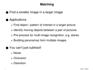

Image Feature Matching Strategies Guide
E N D
Presentation Transcript
Matching • Find a smaller image in a larger image • Applications • Find object / pattern of interest in a larger picture • Identify moving objects between a pair of pictures • Pre-process for multi-image recognition, e.g. stereo • Building panoramas from multiple images • You can’t just subtract! • Noise • Occlusion • Distortion
A simple matching algorithm • For each position / location / orientation of the pattern • Apply matching criteria • Local maxima of the criteria exceeding a preset threshold are considered matches
Match Criteria: Digital Difference • Take absolute value of pixel differences across the mask • “Convolution” with mask * -1 (match causes 0) • Not very robust to noise & slight variations • Best is 0, so algorithms would minimize rather than maximize • Very dark or very light masks will give larger mismatch values!
Match Criteria (Correlations) • All are inverted (and 1 is added to avoid divide by 0) • C1 - use largest distance in mask • C2 - use sum of distances in mask • C3 - use sum of squared distances in mask
Correlation: Weighted Summed Square Difference • Create a weighted mask. w(i,j) is a weight depending on the position in the mask. Multiply each weight by the square difference, then add them up. Sample weights (Gaussian) Source: www.cse.unr.edu/~bebis/CS791E/Notes/AreaProcess.pdf
Matching Strategies • Brute force (try all possibilities) • Hierarchical (coarse-to-fine) • Hierarchical (sub-patterns; graph match) • Optimized operation sequence • Short-circuit processing at mismatches for efficiency • Tracking (if possible)
Image Features for Matching • Interest points • Edges • Line segments • Curves
Phases of Image Feature Matching • Feature extraction (image region) • Feature description (invariant descriptor) • Feature matching (likely candidates in other images) • Feature tracking (likely candidates in appropriate region of next image)
Interest Points • Points that are likely to represent the same ‘location’ regardless of image • Points that are ‘easy’ to find and match • Example: (good and bad features)
Goals for Point Features • Useful features tend to persist through multiple scales • Texture elements ‘blur out’ and are no longer interesting above a certain feature • Corners tend to remain corner-like (and localized) over a wide variety of scales • Useful features tend to be invariant to rotation or small changes in camera angle • Avoid operators that are sensitive to rotation • Useful features tend to have a stable location • Avoid features in ‘smooth’ areas of the image • Avoid features along (single) edges
Good Localization of Features • Goal: unambiguous feature • Few spurious matches • Match is obviously strongest at the correct point • Result: look for ‘corners’ rather than featureless areas or edges (aperture problem) Figure 4.4
Evaluating Features for Localization • Autocorrelation • Measure correlation between feature patch and nearby locations in the same image • Good features will show a clear peak at the appropriate location • Ambiguous features will show ridges or no peak at all
Derivation of Autocorrelation Method • Equations directly from Chapter 4
Finding Features by Autocorrelation • Compute autocorrelation matrix A at each pixel • Compute the directional differences (derivatives) Ix and Iy • This is done by convolution with appropriate horizontal and vertical masks (derivatives of Gaussians) • For each point, compute 3 values: • A[0][0] = Ix*Ix • A[0][1] = A[1][0] = Ix*Iy, • A[1][1] = Iy*Iy, i.e. a 3-band image • Blur each of the above images using a bigger Gaussian than step 1 (this is applying the w function) • Compute interest measure based on eigenvalues of the A matrix
Finding Features by Autocorrelation (cont) • A has 2 eigenvalues, indicating direction of fastest & slowest change • Features are at local maxima of (smallest eigenvalue) that is above a threshold • See equations 4.10 and 4.11 for alternative measurements • Option: eliminate features that are too close to better ones (Non-maximum suppression)
Multiple Scale Image • Blur with bigger filters to get higher scales (less information) • Box filter = averaging • Gaussian filter is more flexible (arbitrary scales, though approximated) • Represent by ‘radius’ σ • Image is now a ‘pyramid’ since each blurred image is technically smaller scale • Higher (more blurred) images can be downsampled • Fewer pixels -> more efficient processing • Point coordinates in multi-scale image: (x, y, σ)
Matching Higher-level features • Numerical feature vectors (e.g. SIFT vectors) • Elementary geometric properties (boundaries) • Boundary length (perimeter) • Curvature: perimeter/ count of “direction change” pixels • Chord distribution (lengths & angles of all chords) • Complete boundary representations • Polygonal approximation (recursive line-split algorithm) • Contour partitioning (curvature primal sketch) • B-Splines
Components of A Matching System • Match Strategy • Which correspondence should be considered for further processing? • Answer partially depends on application • Stereo – we know where to look • Stitching / tracking – expect many matches in overlap region • Recognition of models in cluttered image – most ‘matches’ will be false! • Basic assumptions • Descriptor is a vector of numbers • Match based on Euclidean distance (vector magnitude) • Efficient Data Structures & Algorithms for Matching
Match Strategy: When do they match? • Exact (numerical) match (NOT PRACTICAL) • Match within tolerance, i.e. threshold feature distance • Choose the best match (nearest neighbor) as long as it’s “not too bad” • Choose the nearest neighbor only when it is sufficiently nearer than the 2nd nearest neighbor (NNDR) Figure 4.24
Evaluating Matching:False Positives and False Negatives Figure 4.22 TPR (recall) = TP / (TP + FN) or TP / P FPR = FP / (FP + TN) or FP / N PPV (precision) = TP / (TP + TN) or TP / P’ ACC = TP + TN / (TP + FP + TN + FN)
Verification • Given model and transformation • Compute locations of model features in the image (e.g. corners or edges) • For each feature, determine whether sufficient evidence (e.g. "edge pixels") supports the line • If enough features are verified by evidence, accept the transformation
Pose Estimation (6.1) • Estimate camera’s relative position & orientation to a scene • Least squares formulation • Given: set of matches (x, x’) and a transformation f(x; p) • Determine how well (poorly) f(x; p) = x’ for all x,x’ pairs • Note: p are parameters of transform • Optimization problem: find p so that the following function is minimized • (Take the derivative of the sum and set it to 0, then solve for p) – see optimization.ppt
Local Feature Focus Method • In model, identify focus features • These are expected to be easy to identify in the image • For each focus feature, also include nearby features • Matching • Find a focus feature • Find as many nearby features as possible • Determine correspondences (focus & nearby features) • Compute a transformation • Verify the transformation with all features (next slide)
RANSAC (RANdom SAmple Consensus) Method • Start with a small (random) set of independent matches (hypothetical, putative) • Determine a transformation that fits this small set of matches • [ Remove ‘outliers’ and refine the transformation ] • [ Find more matches that are consistent with the original set ] • If the result isn’t good enough, choose another set and try again…
Pose Clustering • Select the minimal number of control points necessary to determine a pose, based on transformation • E.g. 2 points to find translation + rotation + scale • For each set of points, consider all possible matches to the model • For each correspondence, "vote" for the appropriate transformation (like Hough transform) • Transformations with the most votes "win" • Verify winning transformations in the image
Problems with Pose Clustering • Too many correspondences • Imagine 10 points from image, 5 points in model • If all are considered, we have 45 * 10 = 450 correspondences to consider! • In general N image points, M model points yields (N choose 2)*(M choose 2), or (N*(N-1)*M*(M-1))/4 correspondences to consider! • Can we limit the pairs we consider? • Accidental peaks • Just like the regular Hough transform, some peaks can be "conspiracies of coincidences" • Therefore, we must verify all "reasonably large" peaks
Improving Pose Clustering • Classify features and use types to match • T-junction vs. L-junction • Round vs. square hole • Use higher-level features • Ribbons instead of line segments • "Constellations of points" instead of points • Junctions instead of points or edges • Use non-geometric information • Color • Texture
Cross Ratio: Invariant of Projection • Consider four rays “cut” by two lines • I = (A-C)(B-D) / (A-D)(B-C)
Geometric Hashing • What if there are many models to match? • Separate the problem • Offline preprocessing (of models) • Create a hash table of (model, feature set) pairs, where the model-feature set has a given geometry • E.g. 3-point sets hashed by 3rd point's coordinate in terms fo the other two • Online recognition (of image) and pose determination • Find a feature set (e.g. 3 points) • Vote for the appropriate (model, feature set) pairs • Verify high-voting models
Hallucination • Whenever you have a model, you have the ability to find it, even in a data set consisting of random points (!) • Subset of points can pass point verification test, even if they don't correspond to the model • Occlusion can make 2 overlapping objects appear like another one • Solution: careful and complete verification (e.g. verify by line segments, not just points)
Structural Matching • Recast the problem as "consistent labeling" • A consistent labeling is an assignment of labels to parts that satisfies: • If Pi and Pj are related parts, then their labels f(Pi), f(Pj) are related in the same way • Example: if two segments are connected at a vertex in the model, then the respective matching segments in the image must also be connected at a vertex
Interpretation Tree (empty) A=c A=a A=b B=b B=c B=a B=c B=a B=b Each branch is a choice of feature-label match Cut off branch (and all children) if a constraint is violated
Constraints on Correspondences (review) • Unary constraints are direct measurements • Round hole vs. square hole • Big hole vs. small hole (relative to some other measurable distance) • Red dot vs. green dot • Binary constraints are measurements between 2 features • Distance between 2 points (relative…) • Angle between segments defined by 3 points • Higher order constraints might measure relationships among 3 or more features
Searching the Interpretation Tree • Depth-first search (recursive backtracking) • Straightforward, but could be time-consuming • Heuristic (e.g. best-first) search • Requires good guesses as to which branch to expand next • (Specifics are covered in Artificial Intelligence) • Parallel Relaxation • Each node gets all labels • Every constraint removes inconsistent labels • (Review neural net slides for details)
Cross Ratio Examples • Two images of one object makes 2 matching cross ratios! • Dual of cross ratio: four lines from a point instead of four points on a line • Any five non-collinear but coplanar points yield two cross-ratios (from sets of 4 lines)
Using Invariants for Recognition • Measure the invariant in one image (or on the object) • Find all possible instances of the invariant (e.g. all sets of 4 collinear points) in the (other) image • If any instance of the invariant matches the measured one, then you (might) have found the object • Research question: to what extent are invariants useful in noisy images?